What do you think is the possibility, when you are choosing and sorting images based on the JPEG previews, that you are going to discard the better-quality image, and keep the lesser-quality one? Let’s take a look at a typical “training” shot for a holiday – noon of a sunny day, blue Ionian sea, bright white limestone pebbles, bushes with dark-green, high-detail leaves (which lose all detail if the shot is underexposed), deep shadows under the bushes. These types of scenes typically have a very wide dynamic range. We will see later, however, that the real range of the shot we are examining is pretty much only 8 EV, if the exposure is technically correct.
Let’s shoot in RAW, bracket the exposure, and try to choose the best shot picking the image the “old” way, which is based on the built-in JPEG, using the JPEG histogram, and the brightness on the screen.
Let’s look at the two shots, one taken at 1/1600 sec, and the other, taken +1.33 EV, at 1/640 sec:
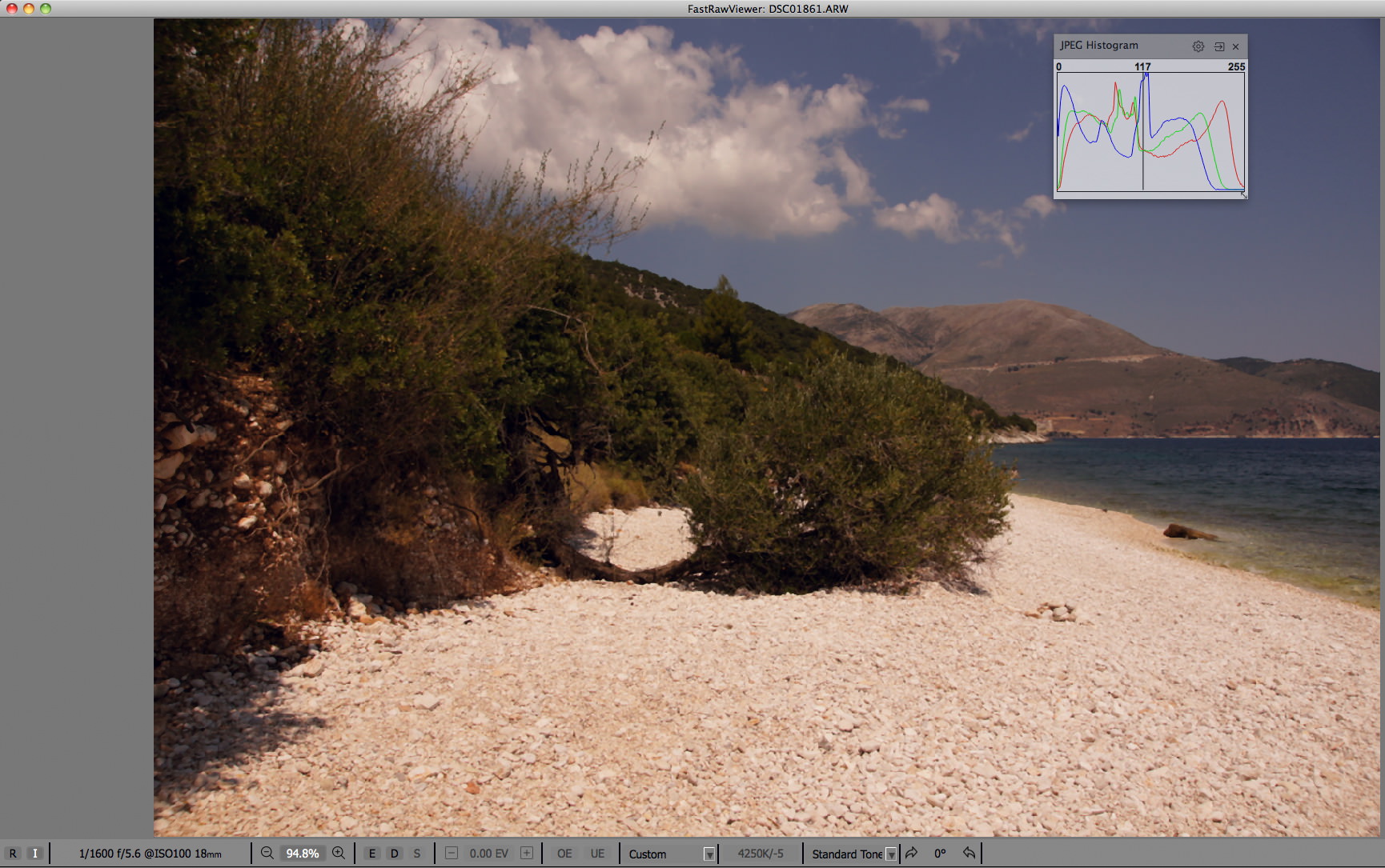

Looking at the JPEG histograms, out of the two shots, the shot #1861 (figure 1), is exactly what we need in terms of exposure (histogram just touching the right wall), while the second shot, #1865 (figure 2), is heavily overexposed on the pebbles and on clouds, lacking plenty of details in those areas; and the histogram for the embedded JPEG of the shot #1865 “climbs the right wall”, confirming what seems to be overexposure.
Now let’s look at the RAW for the same images, setting white balance from a white pebble and using propagation mode so that the next file will be opened with the same white balance we have set for this one.
Consider the RAW histogram and overexposure statistics for the shot that seems to be correctly exposed if looking at JPEG preview:

And now the other one that looked overexposed in JPEG:
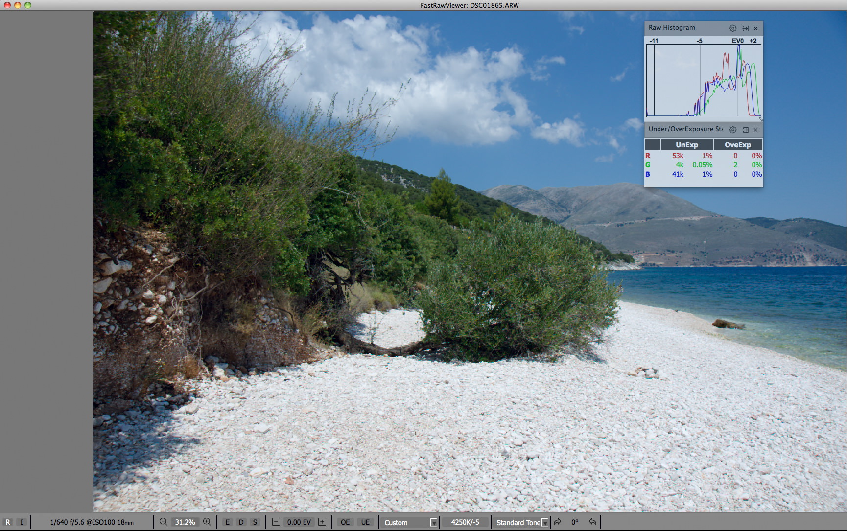
Oops… Examining the RAW histogram for each of the shots, we see that the first one, #1861, that looked properly exposed based on JPEG, is heavily underexposed in RAW (the histogram is shifted to the left, having a substantial gap between the edge of the histogram and the right wall), while the other shot, #1865, is taken using what is often referred to as “ETTR technique” – histogram is all the way to the right, the shot is exposed in such a way that it has nearly no overexposed pixels.
In this manner, when trying to pick an image using JPEG, and not RAW, and making the decision based on the JPEG histogram and on-screen brightness but not the RAW histogram, we have chosen an image that is underexposed by 1.33EV.
Let’s have a look at the next shot #1866, where 1/3 EV is added to exposure compared to already “hot” shot #1865.
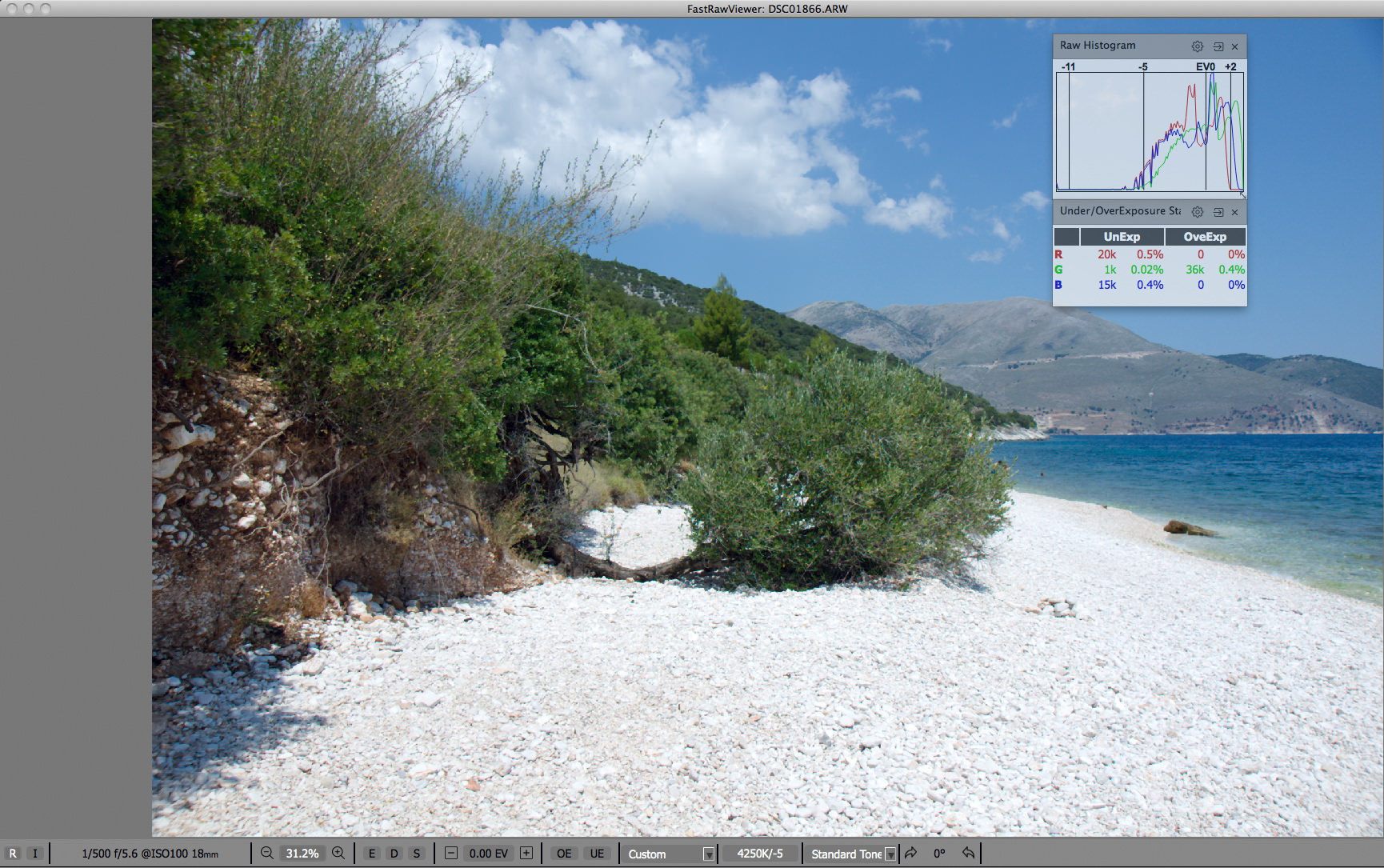
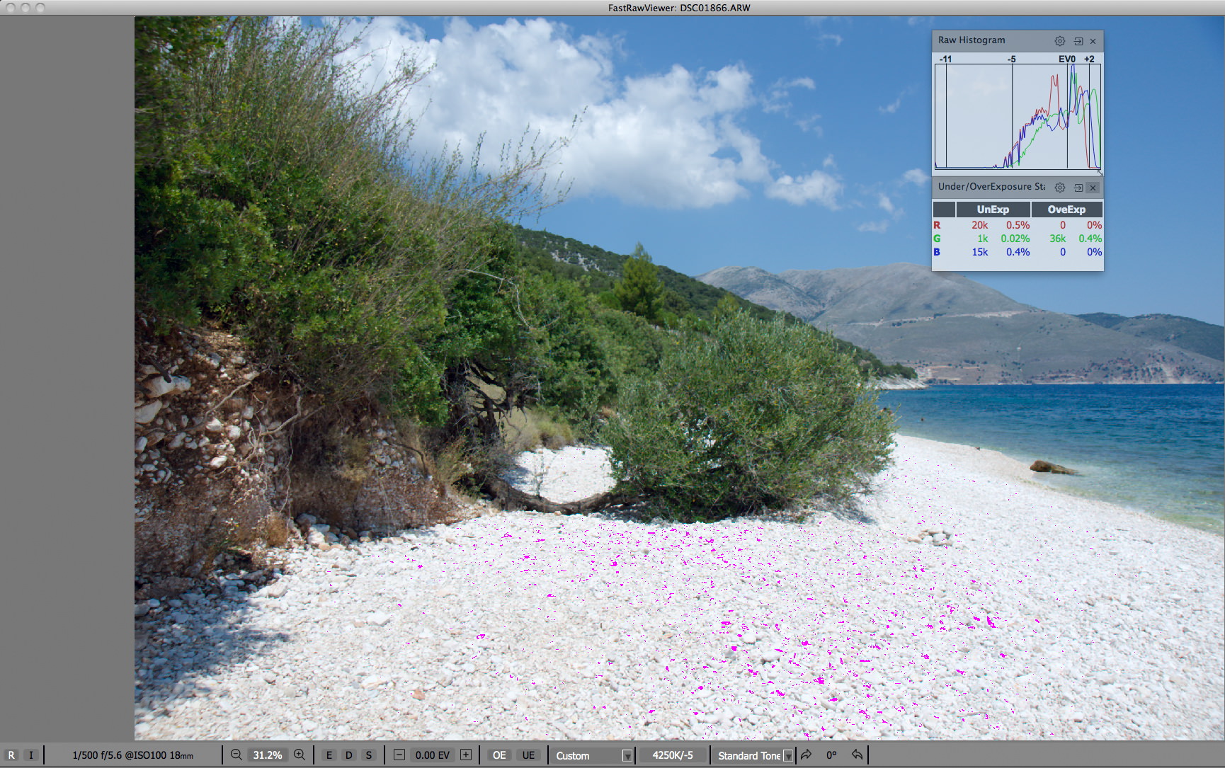
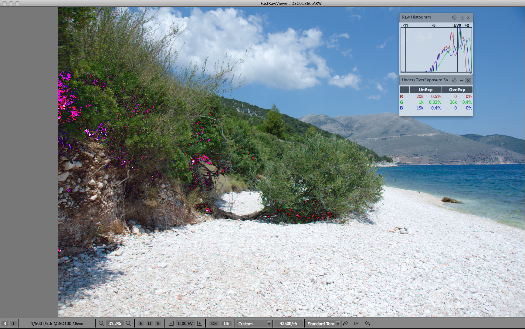
We can see that we have lost very little – only 0.4% of pixels ended up overexposed, and only in the green channel. To see what are the overexposed areas on the shot we press ‘O’ on the keyboard, and magenta highlighting appears on the blown-out areas on the pebbles, below, figure 6.
This small defect is easily fixed in RAW conversion.
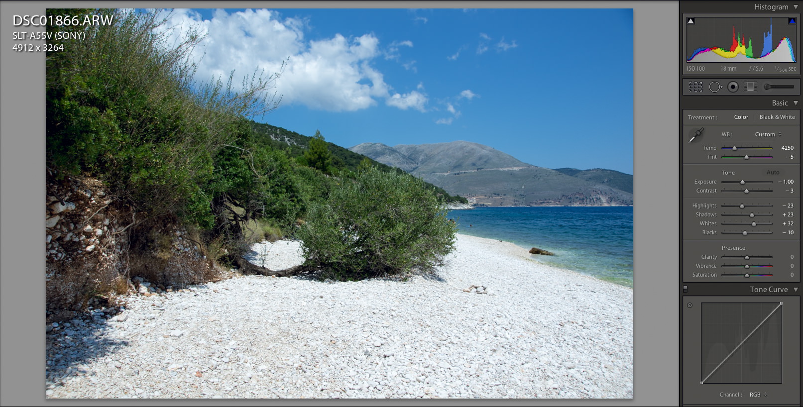
Opening this file in Adobe Lightroom, the white balance is picked from XMP file recorded by FastRawViewer so we do not need to set it again, and pressing the Auto button for the Tone settings, we will get the following very usable image:
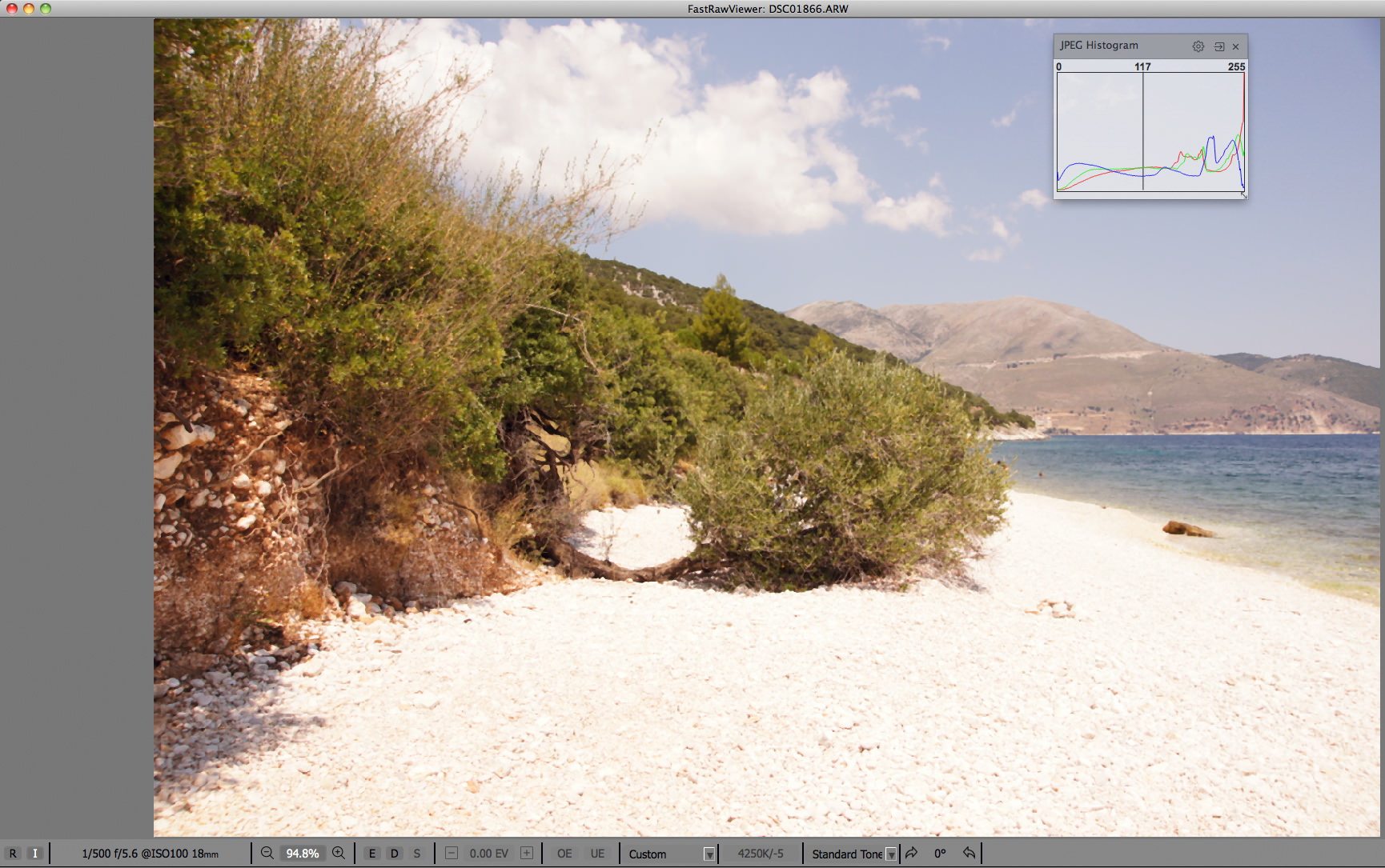
Meanwhile, if we had looked at the embedded JPEG for this shot #1866 and the JPEG histogram, we would have surely discarded this shot, because it looks grossly overexposed, as also indicated by the JPEG histogram climbing the “right wall”:
Take note that based on the RAW histogram for the shot #1861 it appears that we need about 10 EV dynamic range for the camera to render the details in shadows. This is quite optimistic for the given camera, not to mention that for quality and detailed shadow reproduction no more than 8 EV is allowed on the final image.
It turns out that with technically correct exposure, we can place most of the scene in the required 8 EV range during the shoot, without additional work in a converter or graphic editor.
Let’s now explore the underexposure, evaluating the image areas below the 8 EV limit. To display underexposure highlighting we press ‘U’.
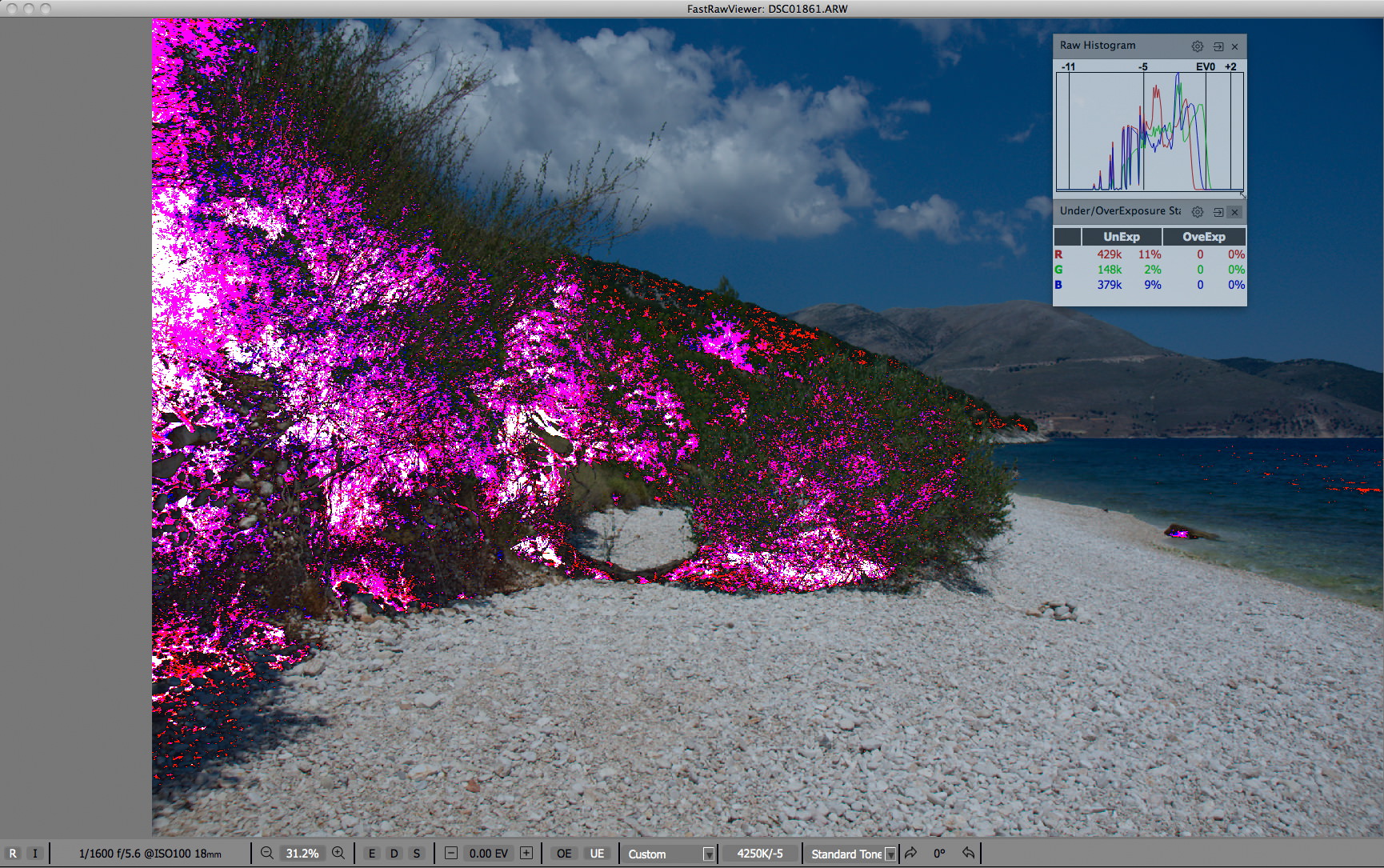
We can see that on the shot #1861, around 10% of the area is underexposed both in the red and blue channels (see the magenta and white highlighting on the figure 9, above), while on the shot #1865 below:

the underexposure zone makes up about 1% of the total image area, which is completely normal.
For the shot #1866 (figure 11), the overexposure zone is a rather negligible 0.5% of pixels.
Now let’s visually analyze the deep shadows for each of the three images.
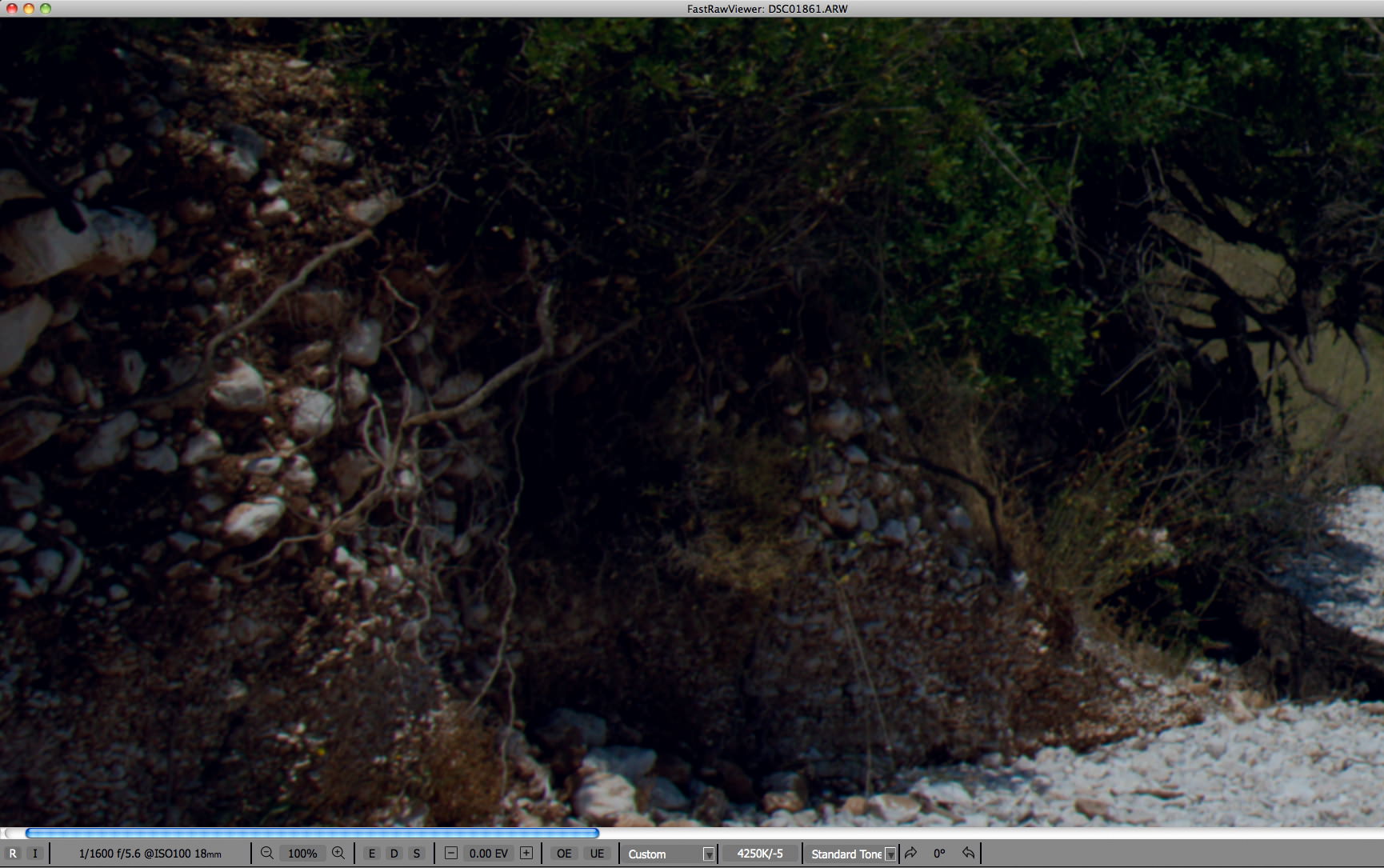
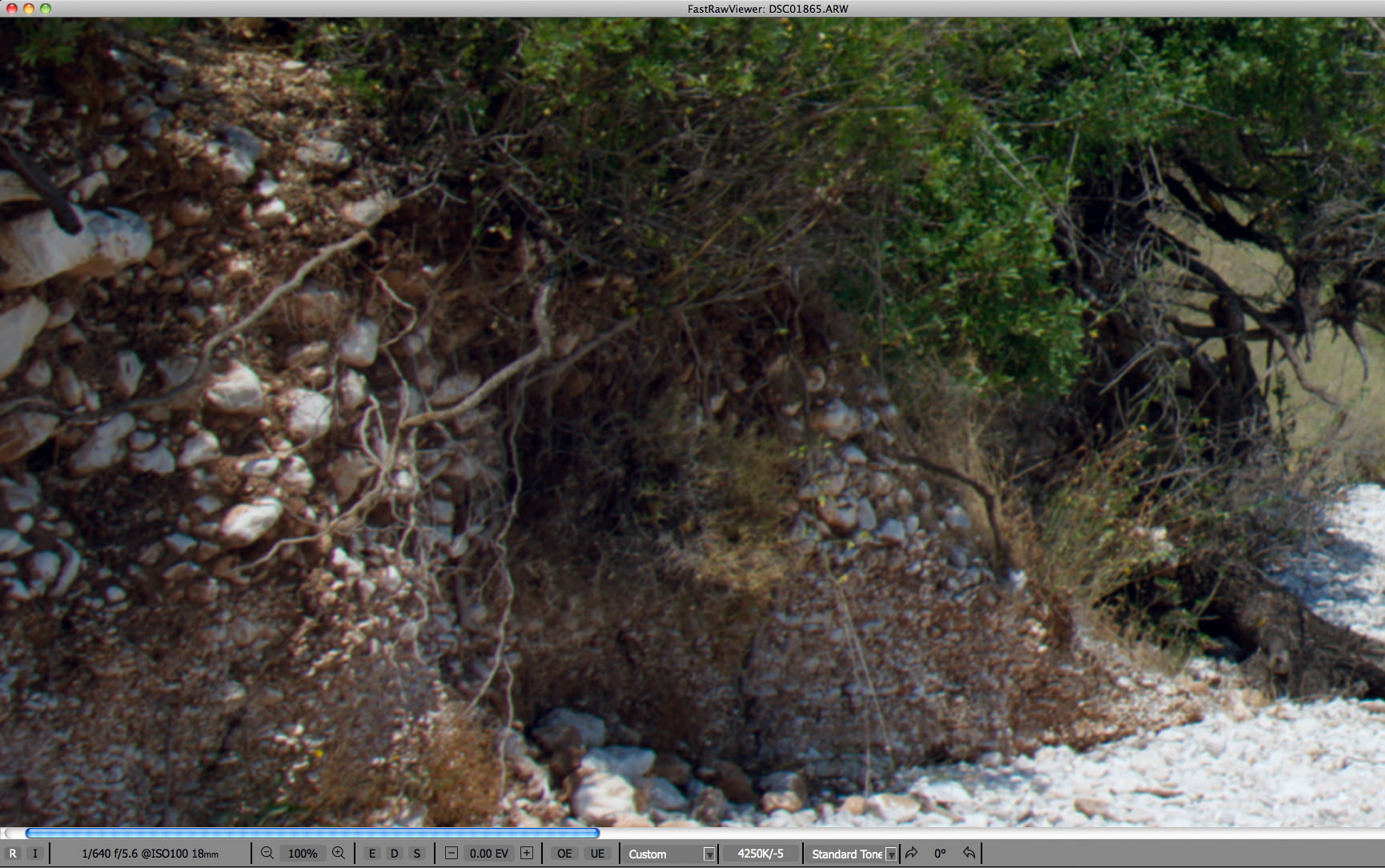
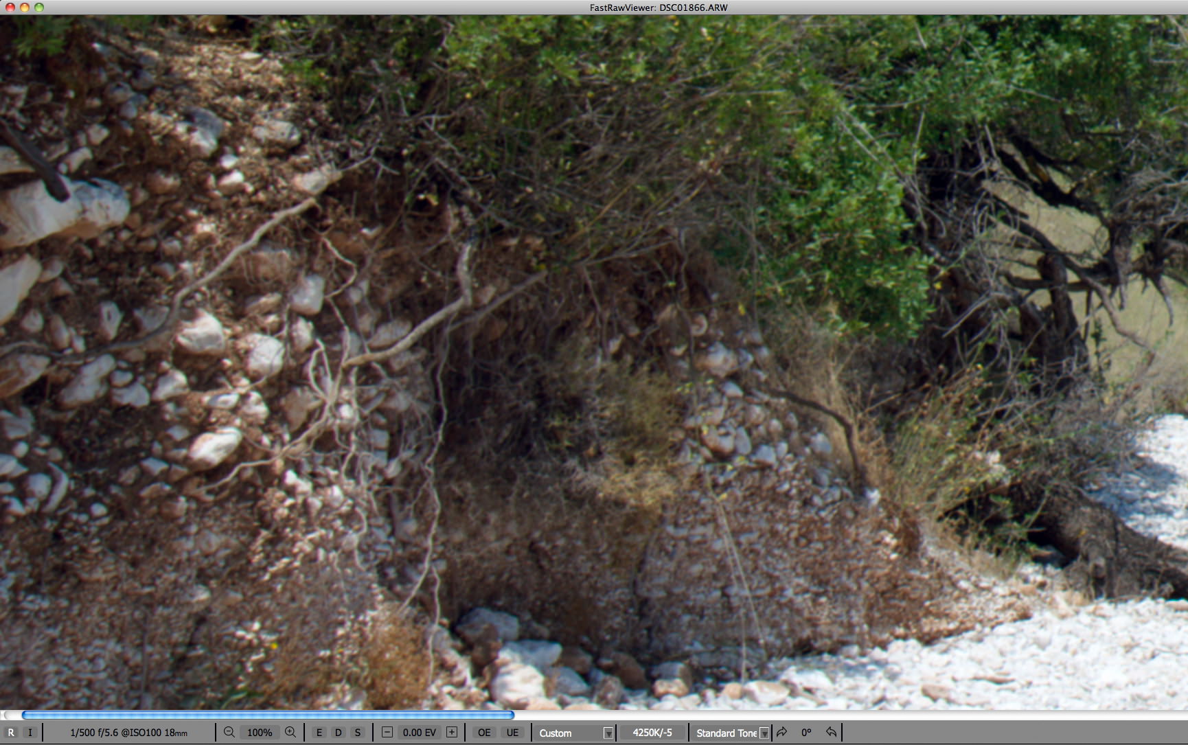
We can see that for the shot #1861 image (figure 12), the details in shadows are plugged to pitch black, while for shot #1865 (figure 13) and especially on shot #1866 (figure 14) they are quite usable. Basing our image selection on JPEGs we would end up with trashing the correctly exposed shots and picking a shot that is underexposed somewhere around 1.5 stops.
As you can see, JPEG histograms can be very deceptive and are no indication of RAW data. So… When culling shots judging the technical quality based on the embedded JPEGs or uncontrolled RAW conversions instead of RAW, you risk making a mistake, especially with difficult scenes having deep shadows, throwing away perfectly good exposures in favor of not so good – because in some sense you are choosing the shots being mislead or even blindfolded.
This is definitely food for thought for my workflow. I love the speed of PhotoMechanic, but now it feels like I’ll be hindering my ability to pick/cull because I really can’t rely on the exposure and histograms in it at all. A lot of my shots are bracketed landscapes so this is a big problem. I might have to go back to doing everything in LR.
Great article. i am struck by how the process you describe is comparable to using the zone system with large format 4×5 film. In both bases there are decisions you make to create the image you want. The process takes time to learn, starts with visualization & measurement of tonal range at exposure, and carries through to production of the image! For landscapes i may start carrying my hand held spot meter again!
I know this is a long-debated topic but I just had to ask this here again, is ETTR the right way to do it? I mean, before knowing about ETTR (which I did after I posted about this on the UglyHedgeHog forum), I’ve always read that it’s always better to underexpose than overexpose. I read that in many articles on PetaPixel, Fstopper (Dani Diamond being one author I remember as of now who recommends this method), and many other places. Especially as I shoot Nikon, and they say Nikons have more dynamic range, it’s better to shoot underexposed because Nikon has more data in the shadow areas.
I was blown out after receiving the responses on my forum topic that it was actually better to over expose, or the ETTR term. After researching on the web I figured out it was yet another debate like Nikon vs Canon or Mac vs PC.
On an article at PetaPixel, an author wrote about how Nikon can retain more data in shadow areas. The comment section was full of Canon shooters saying that Canon does the same thing but with the highlight areas. So if you shot Canon, you’d get more data out of highlight areas. If you shot Nikon, you’d do the opposite.
Now, given that most people shoot Canon, I’m guessing that’s why the ETTR technique was invented? Because Canons retain more data in highlights? Or is that the basic way digital sensors work? I mean, does it matter/differentiate based on what camera I shoot if I were to decide whether to shoot underexposed or overexposed? And, should I shoot underexposed or overexposed in a slightly manner?
Thanks for any help. I’m an enthusiastic photographer with an entry level camera and I can’t get my head around this. Every time I shoot I’m in constant dilemma what to do.
Dear Sir,
This scene must be exposed to the right because of the nature of the scene. It is right with both film and digital.
Light is digitized in such a way that every “right” stop has double the resolution of every subsequent “left” one. Paradoxically human sight is more sensitive to shadows rather than highlights so a proper exposure results in a lot of “wasted” resolution. Pictures exposed to the right will contain more detailed information which translates to better quality at the extremes.
en.wikipedia.org/wiki/…_the_right
Dear Boris,
> Light is digitized in such a way that every “right” stop has double the resolution of every subsequent “left” one
Not so simple. The highlight portion of the working part of photon transfer curve may well be non-linear at base ISO. In that case unwarranted ETTR (that is, exposing a low contrast scene to the extreme right) damages the colour. Another issue arises when a twisted colour transform is used – result is substantial colour difference between the “normally” exposed shot and ETTR shot, with ETTR shot showing wrong colour.
Just downloaded the trial and am impressed with the capabilities. However, the 107 page user’s manual is rather daunting and if this is all about saving time so you can shoot more and fool around less, I think it would be great for you to write a quick tutorial of workflow from camera, through FRV and into LR and post it on Photography Life and/or the FRV site. For instance, do you just plug your camera’s memory card into a reader, open the folder from there and start editing? (I’m impressed at how the RAW images loaded faster than I could scroll if I just viewed them straight off my XQD card.) Can you add ratings to the memory card, sort out only the keepers, then just import those to LR or do you dump all the files on a separate drive, run FRV from that, then import to LR for dng conversion? Is there a grid view of thumbnails possible? What about side by side comparisons of two similar images?
Dear John,
What I do is this:
– cull through the shots on the card and move the images I select to a folder on a hard drive (Shift-M)
– cull through that folder and set labels, ratings, white balance, exposure correction, orientation and if accounting an image I do not want – moving it to _Rejected folder (Shift-Ctrl/Cmd-Del)
– import the resulting folder into raw converter (Lr in your case I guess)
We are working on adding filmstrip. As to comparing several images side by side, we will implement it but it will take some really serious work. Fortunately, after the initial filtering, the shots to compare in that way are not so many and this can be done in Lr.
Here is a map of the workflow involving FastRawViewer and Lightroom
s3.amazonaws.com/Iliah…V_Lr_4.pdf
What I simply don’t understand is why camera manufacturers do not have an Auto-ETTR feature built into their systems if it is the correct way to shoot RAWs. The only article I found that might explain the reason for this omission is the following: howgreenisyourgarden.wordpress.com/tag/expose-right/ Any thoughts?
Dear Hans,
It is impossible to implement ETTR without photographer’s deciding what highlights he can afford to blow out.
This is a very compelling article. It is an aspect of photography I had not considered before. Why camera manufacturers don’t by default show a RAW histogram whilst shooting RAW seems foolish. Thank you for bringing this to my attention.
The new firmware update of the D810 and D750 is going to address thiss, as far as I know.
Dear Jason,
In fact the question is more about exposure meter calibration and in-camera JPEG processing; it is not always possible to look at LCD while shooting, while meter calibration for RAW and JPEGs needs to be different with current OOC JPEG algorithms.
I’m might be complete newbie in this topic and this article is really confusing for me to wrap my head around. It doesn’t have one on one notes to picture correlation that this site follows on other articles. Would be nice to add complete settings under each picture so we get complete idea rather talking about just one factor like shutter speed or EV.
Again it could be me being a newbie or a dummy not able to understand this easy enough on my first read. Will read again once I get home and update comments.
Thanks
John
Please ignore this above comment just found out where to look on the image. Reading in mobile did not see the whole picture. My bad
I am a new photographer and I would like to say that I consult many different mediums for information, and this website is by far the best I go to. So thank you for putting out great content in a colloquial voice.
I am a perfectionist by nature, and this article has me excited because I am mainly having issues with getting things correctly exposed. More than half the time I am not even sure which images are correctly exposed or not. I am confused with the unit of eV’s. I am an engineer, so I know these as the associated energy with the wavelengths of light, but how do they come into play with photography? Like I said, I have only been doing this for a month, so at this point should I even worry about this article?
Currently I do shoot in the raw, and I try and do all my shots in manual mode, or A-priority (at this blogs suggestion, haha). Please let me know! Thanks!
Dear Brandon,
The traditional answer is 1 EV is 1 stop, that is the light change of 2x (2 times). More detailed article can be found at en.wikipedia.org/wiki/…sure_value
Furthermore I have LR, but this FastRawViewer program looks great. Is it worth purchasing this early?
Brandon, it can be confusing at first, but in photography terms EV means Exposure Value, not the science meaning of electronvolt
I glad you posted this article. Its something I noticed quite a while ago. I don’t cull images in camera ( I wait until I load the files into LR ), but I know many people that do. Thanks for posting !!
Very interesting, particularly for many Nikon users as reportedly Nikon will be releasing new firmware for many of it’s cameras which includes adding RAW histograms. The original announcement set the release date as being today 1/19/15. It will be interesting to test it out with your article in mind.