We’ve gotten several emails, the most recent and the best phrased one from a reader of Photography Life, with questions along the following lines:
What happened to my mid-tones? I set the exposure using exposure meter, opened the shot in Adobe Lr (or Adobe Camera Raw, or some other converter) … and the shot looks overexposed and everything from mid-tone and up looks very flat. If I shoot in RAW+JPEG, the JPEG looks OK, while the RAW is not. Should I expose lower?
We’ve decided that the reply to this question belongs here.
Table of Contents
Short Version
Please don’t lower the exposure, you will be underexposing by more than 1 stop in addition to the underexposure due to camera meter calibration. Not a great idea, especially if the light is low and you are already above ISO 400.
As a result of lowering the exposure you will push the shadows higher on the tone scale while doing raw conversion, thus transposing shadow noise and artifacts (such as banding and blotches) to lighter tones where they are more visible; consequently you will reduce resolution in those areas, as more noise and less levels in raw mean less details. Instead, change the default settings (read on for a suggestion) or adjust on a per image basis. Having customized defaults, however, will save you a lot of time down the road. While reading, please keep in mind that one can’t judge the exposure by the brightness. Brightness is the product of the raw conversion process and as such depends on the settings in the raw converter, including the default settings, which may not be so obvious. Of course, brightness also depends on monitor calibration and viewing conditions, as well as the ISO setting in the camera, much the same way the volume control sets the loudness. That, however, is a subject for another day.
First, let’s see how this brightening happens in raw conversion.
Comparing raw rendered “as is” to its default render in a converter
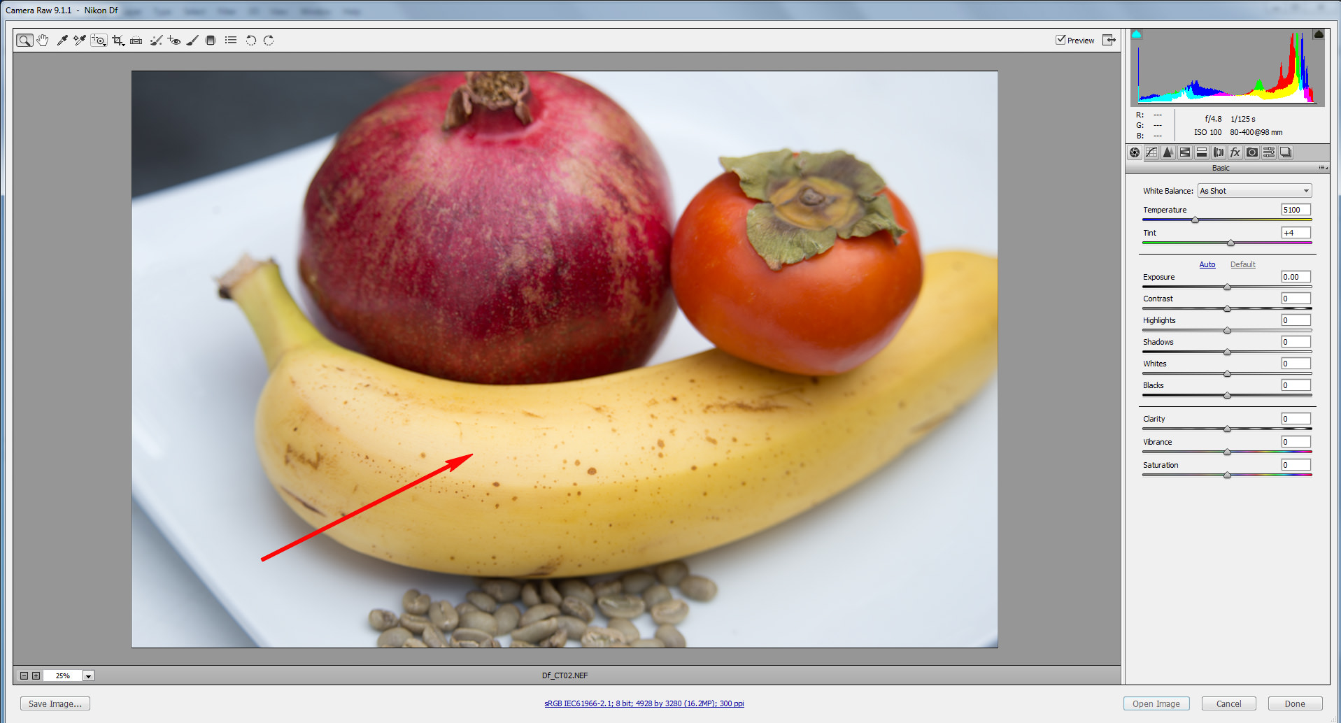
Consider the following example. When opening this shot in ACR or Adobe Lr (and in some other converters, too) it does look overexposed and flat on the higher tones (see the upper left part of the banana: it’s starting to lose volume, look flat, glossy, nearly featureless; the persimmon, conversely, is obviously too bright)
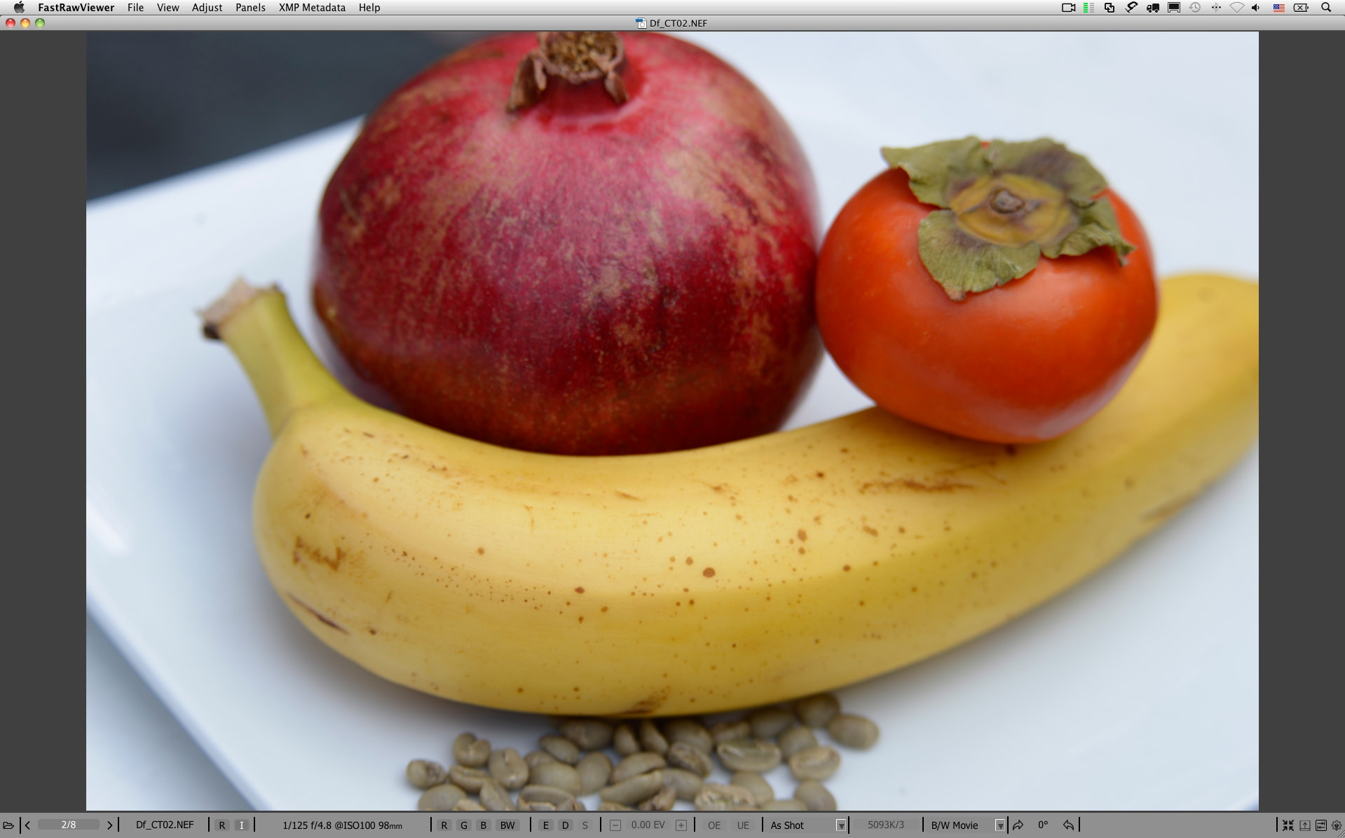
Comparing it to the JPEG the camera recorded, the JPEG looks much less flat in that area (ironically, this is because my cameras are set to custom “flat” picture control, preventing extreme image brightening)
We can look at this embedded JPEG using FastRawViewer. This looks a little better.
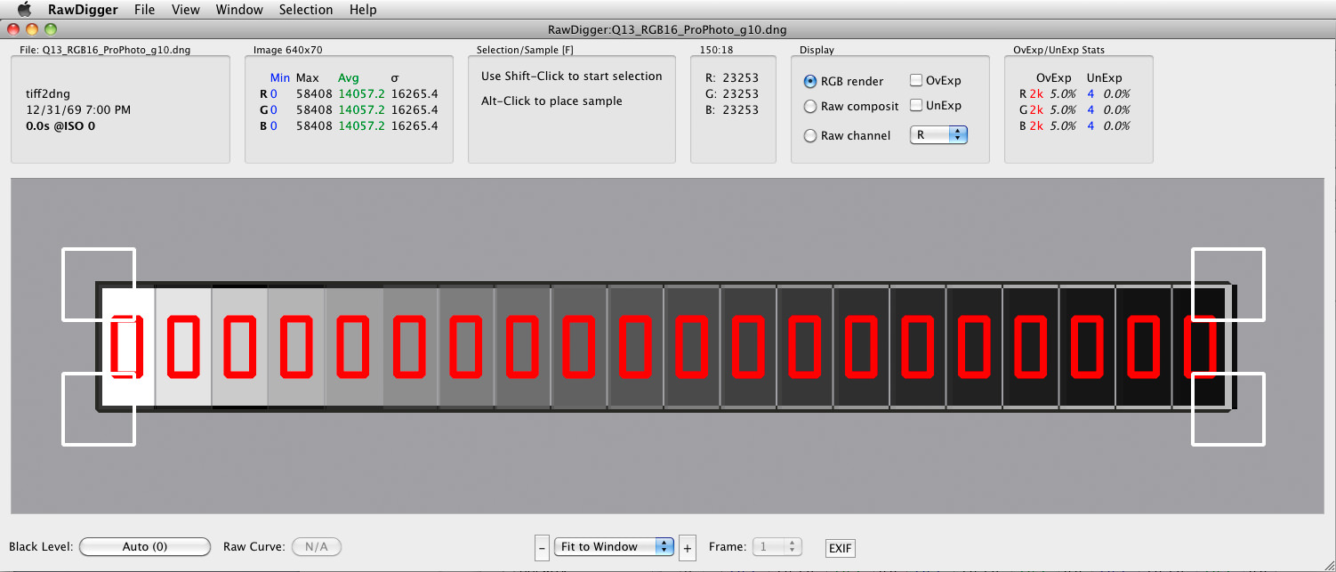
To see the raw truth, we can open the same raw shot in RawDigger, with it being rendered “as is” without any adjustments applied:
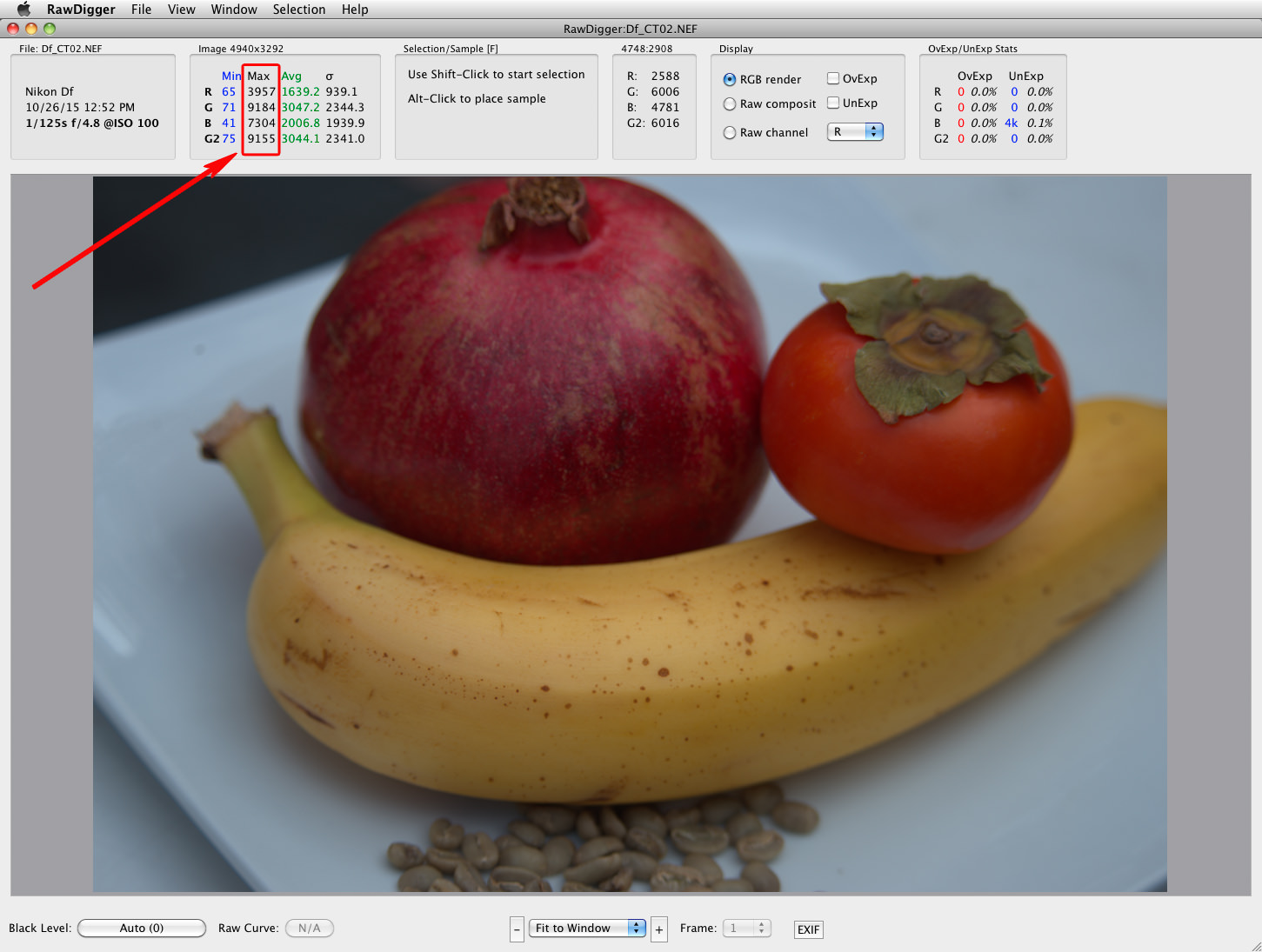
1) The previously marked (Figure 1) area of the shot does not look like it’s been flattened into a pancake anymore
2) The raw statistics and raw histogram indicate that not only is this shot NOT overexposed, as a matter of fact it is underexposed by nearly a stop (the maximum is below 9200 on a 14-bit scale).
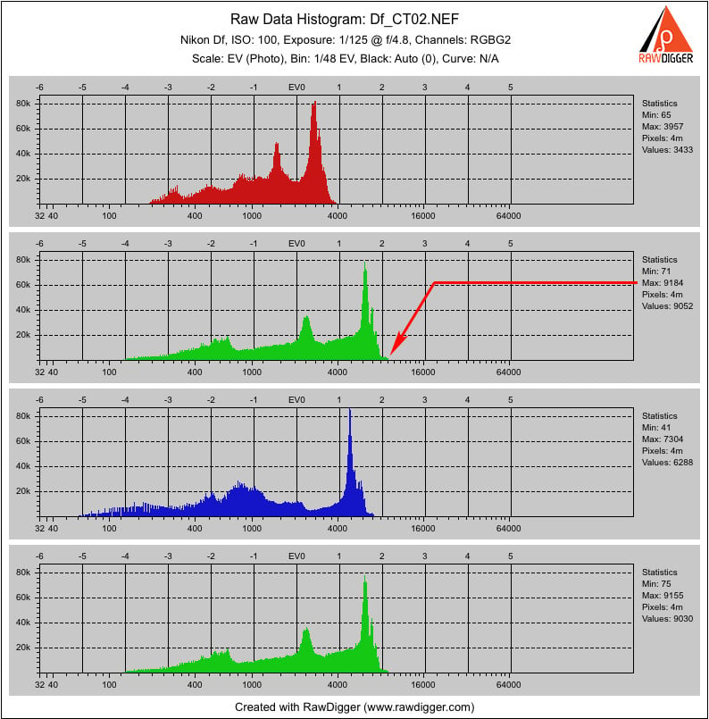
So, if you were to try and expose your shots so that they looked good and properly exposed in a raw converter “as is”, by default, you would need to underexpose this shot even more, close to 2 EV in total.
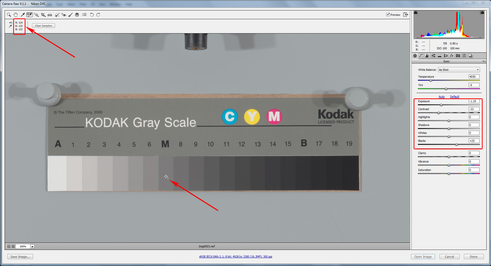
It seems as if ACR (Figure 1) applies some default adjustments to a raw shot upon opening it.
Below we will calculate the exact value of the adjustments that are, by default, applied to the midtone. If you are not into formulas and calculations, you can scroll down to the next part, which is devoted to the practical advice on how to deal with those default adjustments.
Calculating the Brightening Caused by The Default Adjustments
Now, we need something better than just a visual reference, as we are going to be dealing with numbers; we need a shot of a target with known values. The famous Kodak Q13 grey step wedge has known and stable values. It was designed to “find the correct exposure and processing conditions” and suits our situation very well. The Q13 shares first place among the most photographed objects in the world with the Macbeth ColorChecker.
From the Kodak formulation, the absolute reflection density Dr (we will shorten it to just “density”) of the “A” patch is 0.05D, the step between patches is 0.1D. According to the formulation, the “M” patch receives a density of 0.75D (0.05 + 7*0.1D).
Following “A Guide to Understanding Graphic Arts Densitometry” by X-Rite, p.5:
D = log10(1/Rf ), that is Rf = 1 /10^D, (1)
where Rf is Reflectance factor (say, 0.18 for 18%)
More details can be found in ISO 5-4:2009, but the above is sufficient for the task at hand. The Q13 is designed in such a way that the reflectance of the “M” patch as a percentage (clipping point is considered to be 100% reflectance) is very close to the proverbial 18% mid-tone:
100% / (10^0.75) = 17.78%
This is fortunate, as ISO Standard 12232 “Digital still cameras — Determination of exposure index, ISO speed ratings, standard output sensitivity, and recommended exposure index” defines the midpoint on a rendered image as 18% grey.
To connect the dots, let’s also see how to convert density D to familiar photographic stops; that is, to EV units. Given that for linear data:
EV = log2(1/Rf) (2)
Hence, using formula (1), we infer that the correlation between the density and EV units is:
EV = D * log210 ≈ D * 3.322 (3)
That is 1.0D ≈ 3 1/3 stops.
Thus, 0.1D ≈ 1/3 EV (this means that the step between the patches on the Q13 is very close to 1/3 EV), and the absolute density of 0.05D for the “A” patch is ≈ 1/6 EV. For the “M” patch, the absolute value of 0.75D translates to 0.75D*log2(10) ≈ 2.49 EV.
What we learn from the above is that as soon as the “A” patch is slightly (around 1/6 EV) below clipping, the “M” patch is about 2.5 stops below clipping.
Working in RGB, we can calculate the reflectance factor for a channel (channel here is R, G, or B) like this:
Rf = Measured Channel Value / Max Channel Value,
where Max Channel Value is 255 for 8-bit spaces, but for a camera/sensor it is the clipping point
We can express the mid-tone, using the following formulas for RGB space with a gamma (typical gammas: 2.2, 1.8, etc.):
a. as a percentage of the reflection, %
Mid-toneChannel,% = ((Channel Mid-tone Value / Channel Max value) ^ gamma)*100% (4)
b. in photographic stops, EV:
Mid-toneChannel,EV = log2((Channel Mid-tone Value / Channel Max value) ^ gamma) (5)
For the sake of convenience, we will be using Green channel values, as those are unaffected by the white balance. Let’s examine a shot of the Q13 step wedge to find what real values for the mid-tone we got in the shot, so as to compare them further with the converter’s output. Opening the shot in RawDigger, we can see that it contains small blown-out areas of specular highlights.
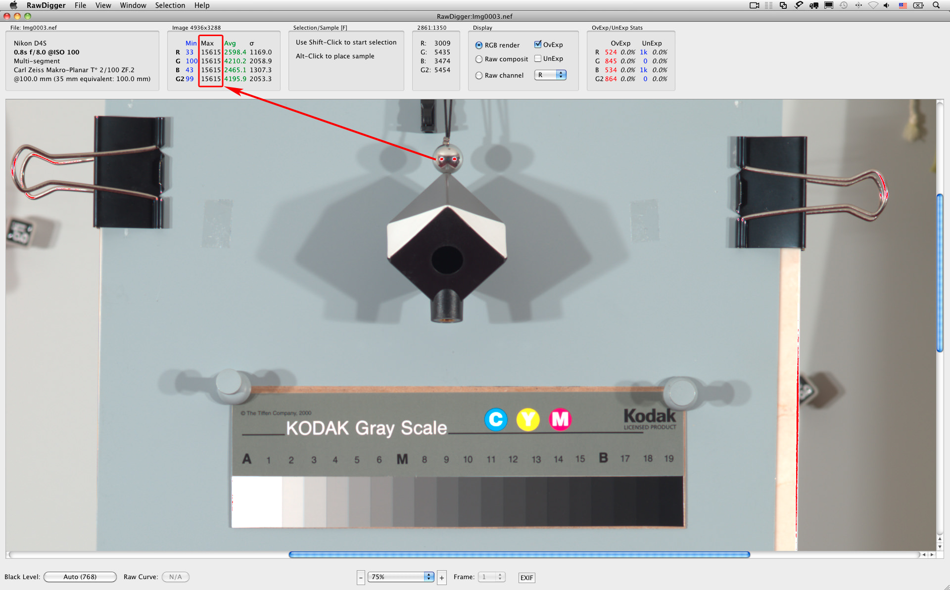
The values for those blown-out areas reach the maximum available for the camera at the given ISO, so we can take the maximum value from the statistics, this value being 15615 (you should not expect it to be exactly 16383 – 2^14-1). By the way, we are sure that the areas are blown out also because the readings in all 4 channels, RGBG, are not only high, but very close to each other too – they hit the hard limit.
This shot was exposed in such a way that the brightest patch is close to clipping. Making a selection over the “A” patch, we can see it is 14209.4, which, according to formula (5) and taking into the account the gamma for the raw data = 1 (the raw data is linear), is log2(14209.4/15615) ≈ –0.14 EV from clipping (1/6 EV is ≈0.17 EV).
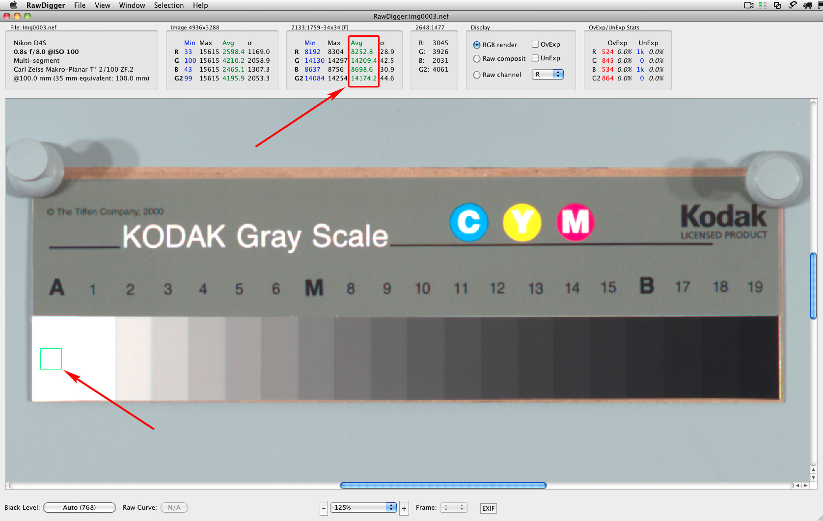
Next, let’s check the value of the “M” patch with RawDigger. A selection over the “M” patch results in an average value of 2755.8.
As we can see, the “M” patch on the shot is very close to the academic mid-tone of 18% and to Kodak’s formulation of 17.78% (see above) – from formula (4); again, using gamma=1 since it is linear raw data, we have:
2755.8 / 15615 *100% = 17.65%
As was already mentioned, ISO standard 12232 calls for the midpoint on a rendered image to be 18% grey, corresponding to the value of 118 in 8-bit (0..255) sRGB within the margin of ±1/3 EV. To convert this interval into photographic stops we use formula (5) with gamma 2.2
log2((118/255)^2.2)±1/3 EV = -2.45 ± 1/3 EV
This means that in photographic stops, the interval for the midpoint is between -2.12 EV and -2.78 EV
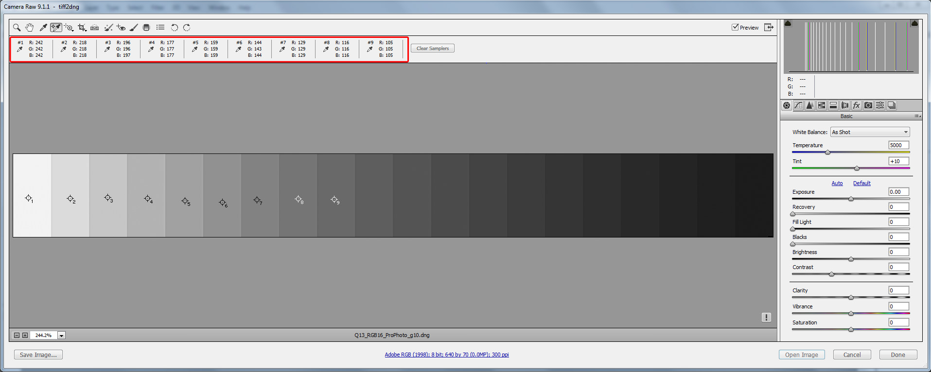
To get back to RBG values we have to repeat the same calculations in reverse, and, to spare you the details, the result is that we should expect the midpoint to be between 105 and 130, accounting for ±1/3 EV tolerance the standard suggests. Now, let’s open the image in Adobe CameraRaw and check the value of the “M” patch.
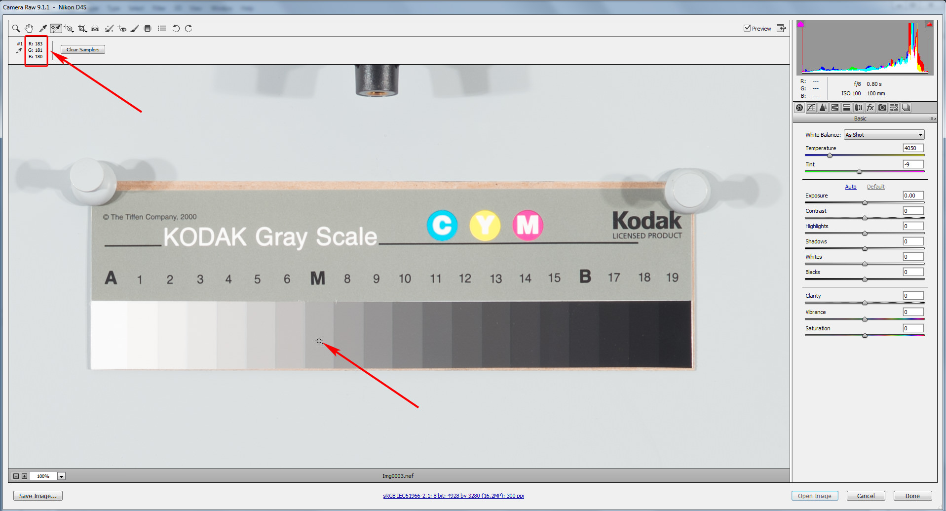
It’s 181 in the Green channel in sRGB, pretty far from the midpoint (if you are using Lightroom, you can turn SoftProofing on and set it to proof to sRGB to see the RGB numbers on a 0..255 scale). But how far is it in photographic terms, that is to say in EV?
Let’s make some calculations, taking into account that the standard says that gamma = 2.2 for sRGB:
The standard calls for 118 RGB for “M” patch, so according to the standard the reflectivity on “M” patch should be (using formulas (4) and (5)):
((118/255)^2.2)*100% ≈ 18.4%
log2((118/255)^2.2) ≈ -2.44 EV (2.44 EV down from clipping)
On our shot the “M” patch is 2755.8 in Green channel (see Figure 8); the maximum value is 15615; and gamma=1, so the reflectivity of the “M” patch from the raw data is (using the same formulas):
(2755.2/15615)*100% ≈ 17.65%
log2(2755.2/15615) ≈ -2.5 EV (2.5 EV down from clipping)
As we have already mentioned, the “M” patch is very close to the academic mid-tone of 18% and to Kodak’s formulation of 17.78%,
After raw conversion, we got 181 RGB for the “M” patch:
(181/255)^2.2)*100% ≈ 47% (instead of 18%)
log2((181/255)^2.2) = -1 EV (1 EV down from clipping, instead of 2.5 EV)
This means that the mid-tone is bumped by about 1.5 EV! No wonder higher mid-tones start to look featureless: they are heavily compressed through a very long and flat shoulder of the default tone curve. This actually means that if you were to try and expose in such a way that the defaults in a raw converter place a mid-tone where it belongs on the default rendition, you might end up underexposing by more than 1 EV — just start decreasing the Exposure value and watch how 118 appears in the green channel when the slider is at -1.2 EV.
This might be not so detrimental when light is aplenty and you are keeping ISO low, but in dim light with exposure going down and ISO going up, you will heavily deplete the camera’s dynamic range.
Practical Part: How You Can Override Default Adjustments
Let’s see if we can change the defaults in such a way that no hidden brightening will happen during raw conversion. Such defaults are easier to set using Process Version 2010. Let’s switch to it. Default settings are now: Brightness = 50, Contrast = 25, Blacks = 5, and Medium Contrast curve. So, one can immediately see that some adjustment have been made to a shot.
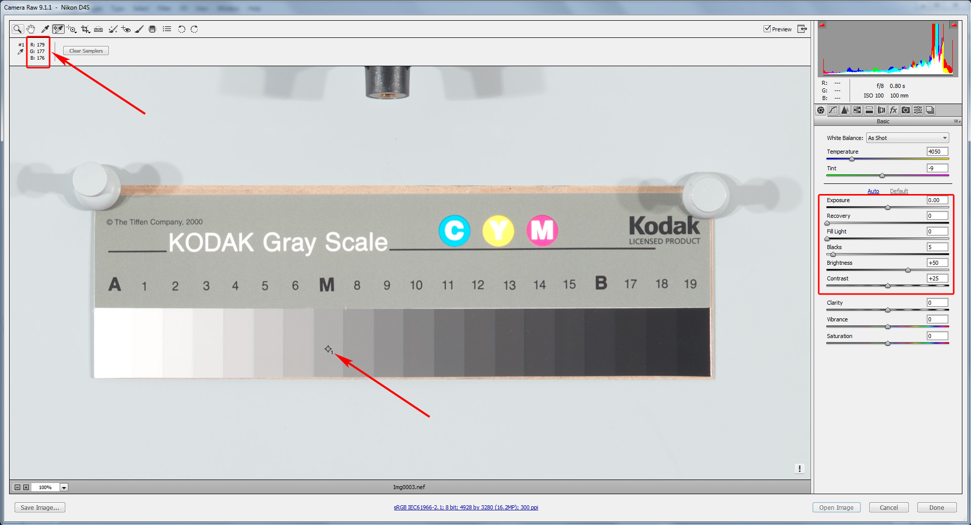
Just on a side note: the selected point of the “M” patch with the default render of this shot of the Q13 in the ACR process 2010 has a value of 177 in Green channel, while for the default render with process 2012 the value for the very same point was 181.
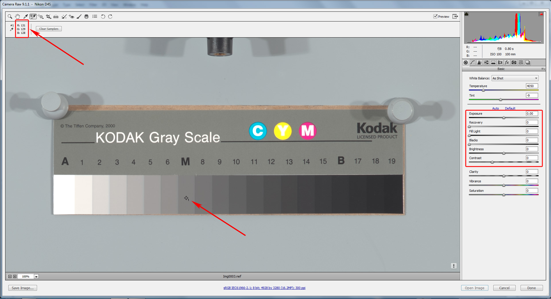
As some of our readers may know, Dan Margulis advocates starting with the zeroed-out rendition; and only then adjusting the sliders to choose the proper settings for conversion; or, better yet, converting with zeroed-out settings and continuing in Photoshop.
Setting the Black, Brightness, and Contrast sliders all to zero, and dropping the curve to Linear, we see that the “M” patch value now becomes 129, that is, according to the standard, in the ballpark for a mid-tone. However, only in its upper margin.
Switching back to Process Version 2012, you can save the resulting settings and use them for zeroed-out renditions – as you can see, now, the “M” patch has a value of 133 in Green channel, placing it very close to where the mid-tone belongs.
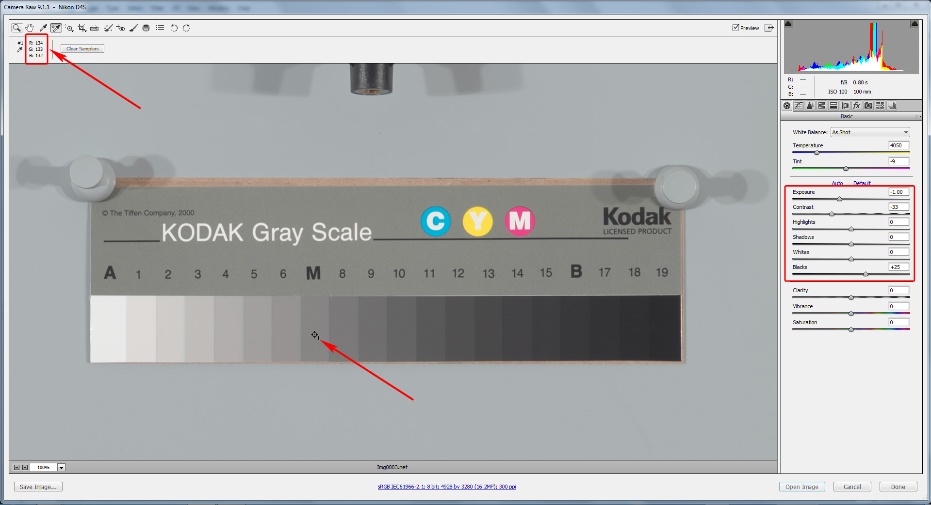
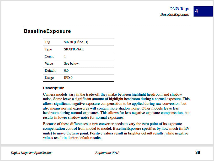
Nevertheless, for process 2012 we are slightly above the standard upper margin, and for the 2010 we are just a little below it. Why? Remember when we discussed the silent/hidden exposure compensation Adobe applies? This “BaselineExposure” (BLE) happens to be 0.25 EV for Nikon D4s for this ISO. Subtracting it from the Exposure, we see the sRGB number in the green channel dropping to 119 for process 2010 with zeroed out defaults.

…and 123 for process 2012 with zeroed-out defaults.
Voilà! Now, with these settings, we have the mid-tone placed correctly, within the tolerance allowed by the standard.
Some Words About BaselineExposure
We already touched upon this subject a year ago in the article “Adobe’s Silent Exposure Compensation“. Another way to look at BaselineExposure is this: BaselineExposure indicates the difference between the clipping in the raw converter and the clipping in the raw itself. BaselineExposure is the amount of EV to which the highlights can be brought back (un-clipped) before “highlight recovery” (that is, the interpolation that reconstructs the clipped channels based on the channels that are not clipped) kicks in.
Referring to certain cameras, some folks say that those cameras allow one to “restore clipped highlights” better. But those highlights they are restoring are not clipped in raw; they are clipped in a raw converter: that is, no restoration happens, just smoke and mirrors. The price for this “feature” is straightforward underexposure, resulting in more artifacts and noise – the lower the camera metering system is calibrated, the lower the exposure, the more headroom in highlights there is for “restoring”, and the higher the BaselineExposure number.
But I digress…
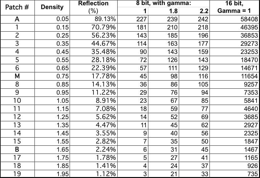
To be sure of what is happening, we’ll use a synthetic dng with a simulated 16-bit Q13 step wedge. The simulation is based on the above-mentioned Kodak formulation; “A” is 0.05D, and each next step adds 0.1D (in other words, the step is 1/3 EV). The BaselineExposure for this DNG is 0, because of how we created that synthetic dng.
Using a superposition of formulas (3) and (5) we will get the RGB value for every patch calculated based on its density:
RGBpatch = RGBMax/10^(Dpatch/gamma) (6)
Based on this formula we can calculate RGB values for every patch of the Q13 for RGB color space with various gamma values.
Now we open our synthetic dng with simulated 16-bit Q13 step wedge in RawDigger,
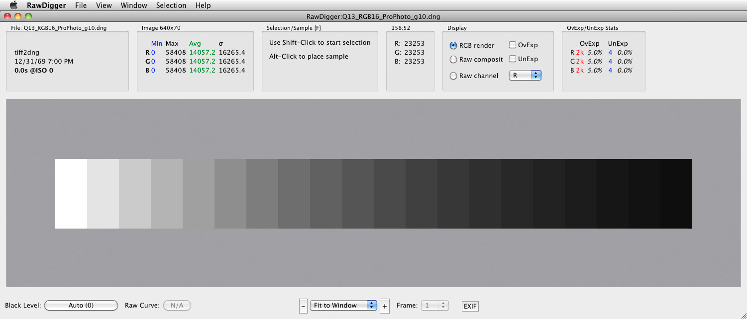
…make a selection grid,
…and save the selection’s RGB values as a table (Excel-compatible .CSV):
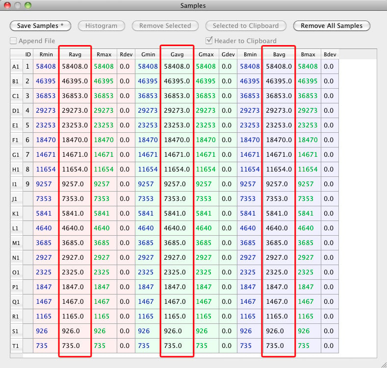
Comparing the numbers calculated (Figure 16, last column – since we have 16-bit linear data) to the numbers in RawDigger (Figure 19) you can see the synthetic dng step wedge is correct. Now, if you open our synthetic dng in ACR (using the process 2010 as more obvious and precise), zero out the settings, place color samplers to 9 patches (unfortunately, ACR allows only up to 9 color samplers at once) and compare the numbers with the table on Figure 16 (please use the appropriate gamma column, 1.8 for ProPhoto, 2.2 for AdobeRGB and sRGB; the numbers agree best for ProPhoto RGB and AdobeRGB due to true sRGB not exactly being the gamma 2.2 space, which affects mostly shadows), you will see that the numbers are very close to what they should be.

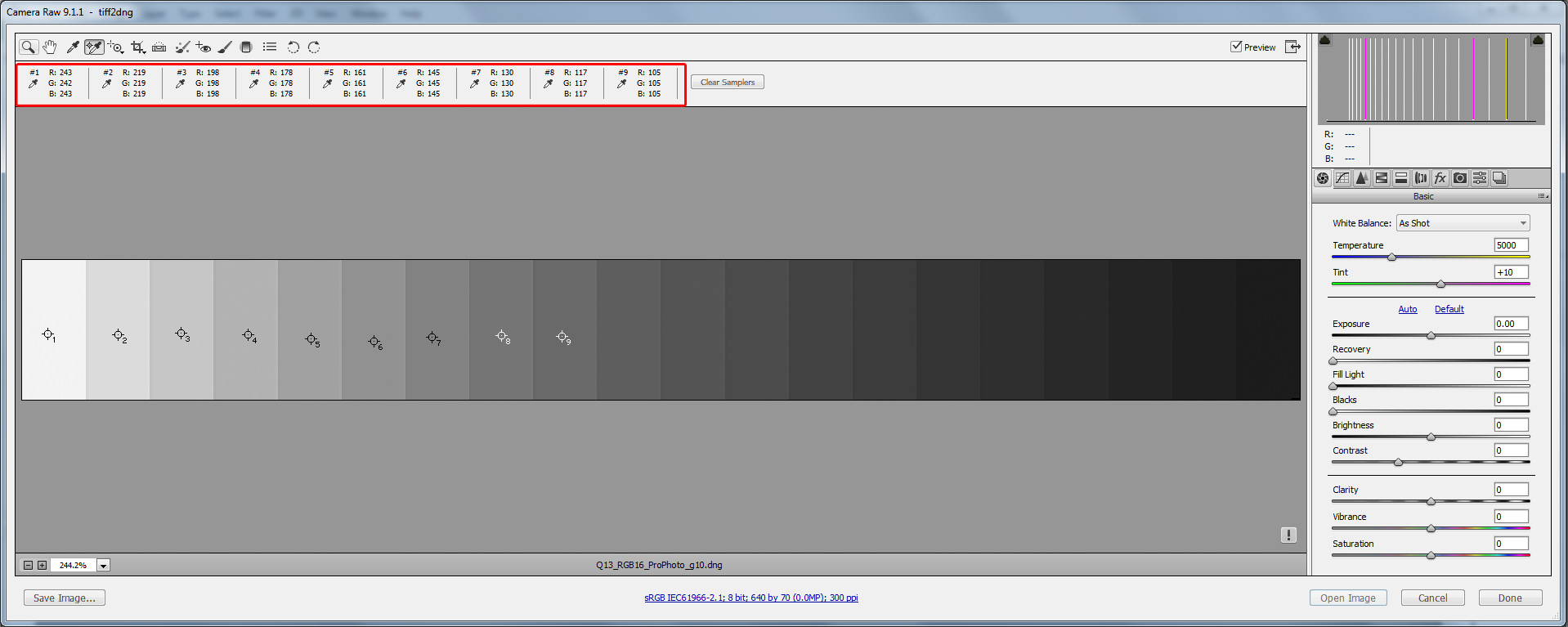
This proves our statement that after we zeroed-out defaults in Adobe raw converter we get accurate scene reproduction, within the BaselineExposure compensation.
In the next article we will show you how to calculate BaselineExposure for your camera using RawDigger.
Thanks for the speedy reply, Iliah,
I have opened various files up and can confirm that RawDigger and Capture NX2 show very similar clipping points.
The problem is the camera is showing clipping too early.
The above is not possible as you can not apply exposure compensation in Nikon Control, only adjustments of the curves (and brightness which is useless and not worth mentioning).
The only way to adjust the in camera blinkies is to adjust the highlight point of the curve, save it and load it into the camera and view the same image again, rinse and repeat until the blinkies are only just starting to appear as a good point. This is what I believe you are suggesting in the link above, tedious but only needs to be done once so well worth it!
The other option is to use Capture One with the ‘Linear Curve’ but I have yet to test this against ACR and Nikon Capture NX2, I will download a trial version later and test this vs ACR and Capture NX2 to see if that ‘Linear Curve’ is indeed giving a flat RAW file with no hidden adjustments.
To my surprise, after testing both ACR and Capture NX2 I discovered that both are giving almost identical files when we apply your Adobe defaults with baseline exposure applied in ACR.
I will let you know the outcome of my testing vs Capture One later.
Many thanks, Iliah!
Hi illiah,
Great article! I have my Nikon d800e set to linear and prefer to use capture NX 2 as my RAW converter. Although capture NX 2 histogram matches the camera histogram, Adobe camera RAW using your suggested defaults is allowing me to push the exposure by at least 1 stop.
Is there a way to achieve similar results using Capture NX 2?
Also there is a n option in Capture One that allowed a linear tone curve which seemed to give a great flat RAW file. I’m not sure if that option still exists, are you aware of it?
Maybe that is a better option that Adobe Camera Raw? At least until I get a Mac.
Dear John,
Nikon are providing for a custom curve in the camera which is useful for ETTR practitioners, have a look at the discussion here: www.dpreview.com/forum…t/58127596
If such a curve is not loaded into the camera, first take a shot that has some area close to clipping, check with RawDigger, readings in green channels of about 15000 in 14-bit mode is what you are after. Load the shot into Nikon Capture and apply the negative exposure “compensation” in NC until the area is un-clipped – the value of the compensation is what you can additionally apply in the camera after the green channel starts to touch the right wall on the in-camera LCD.
CaptureOne still offers the “linear curve”.
Hi Iliah, your are right, Canon (all cameras) and the Nikon “workhorses” are an exeption and there might be a small loss in image quality if underexposing by default + correcting exposure in post. If the needed ISO is above base ISO underexposing might nevertheless be someting to consider if you are not in a totally controlled environment as the risk to loose highlight is much lower + you are not really loosing that much image quality – especially if you are using an “almost ISOless” body.
If I have the time I use spotmetering on the brightest area of my image and use the headroom according to the DxO-calculations, if not or if I can’t risk to loose details in the bright areas (i.e. weddings) I prefere a bit of underexposing (which as you have already proven is more or less a default setting of all cameras), same if the lightning changes quickly (i.e. concerts).
As I use a DSLM (Sony a7II) I am struggling quite often with the over exposure warning of the camera as this is based on the jpg-settings and not on the raw file (as are most histograms on the camera screens) Guess Leica uses a “raw”histogram and Nikon adressed the issue?
> Canon (all cameras) and the Nikon “workhorses” are an exeption and there might be a small loss in image quality if underexposing by default + correcting exposure in post
It is far from being small.
One additional comment: For most cameras using a Sony sensor (many Nikons, Sony, Fuji, Pentax) underexposing is no problem if you are above base ISO anyway as the sensors are “ISOless” and it doesn’t matter if you are correcting the exposure in the post or directly in the camera if you are shooting raw. The Df is one of the few Nikon cameras which is not ISOless, with it you should always try to get the exposure “right” while shooting
Not only “ISO-less” is more of an abstraction (if you check noise levels and shadow non-linearity, very few cameras actually a close enough to ISO-less), all current Canon dSLRs can’t be considered ISO-less, and “few” Nikon bodies which are not ISO-less include current pro workhorses D3s, D4, D4s.
If using spot-metering you could use the DxO “measured ISO” to calculate your headroom. DxO calculation include the common 2,5 EV headroom with an addition 0,5 EV “safety” headroom. If doing the calculation for the D750 at ISO 100 ( www.dxomark.com/Camer…asurements ) the measured ISO is 73.
Now it’s log2(100/73)=0,27 EV -> 2,5EV + 0,5 EV + 0,45 EV =3,45 EV.
For the Df it is 2,5EV + 0,5 EV + log2(100/74)=3,43 EV
For a Olympus E-M1 at Iso 200 it’s 2,5 EV + 0,5 EV + log2(200/122)=3,71 EV
Depending on the camera the headroom might be different for different ISOs
log2(100/73)=0,454
On a side note, there is always a danger that using somebody’s data without understanding what happens and why and without means to verify the data more harm than good can be done.
Thank you, I forgot to play with that setting in lightroom. I like neutral a lot! I had adobe standard as my default when importing pictures and it is way too contrasty! Blowing highlight and increasing shadows too much! It is way easier to make a nice blurry background(soft) that is not distracting with neutral preset.
Iliah, Thank you so much for spending the very many hours it must have taken to properly answer the Photography Life reader emails to which you were responding.
I fully understand that many readers baulk at articles (and comments) that must include the associated mathematics required to properly answer technical questions. I would like to humbly remind the readers of Photography Life of two things that, I think, are essential to the purpose of this website:
1. When you visit a public library, and browse its materials at your leisure, on your way out do you announce to the librarians and the visitors something along the lines of: Your book on steam engines by James Watt included far too much mathematics, I hope you won’t be adding any more books to this library that I find boring to read.
2. Please try hard to remember that you are not obliged to read every book in a library, and that many of the books added to the library are for the education and/or enjoyment of people other than yourself.
Great article! Very well done!!!!
Sorry, I can’t resist: And us poor colorblind people look at all of this and ask: “Just what was the problem with the picture in the first place? I can’t see any issue that needs to be addressed.” Not to mention, depending on the color calibration of your monitor, even color sighted (is that the right term?) people might not see any issue with the picture.
Interesting article, but I believe most of us would like a quick two to three step solution. As a former programmer I enjoy the math, but I also know that most people don’t give a BLEEP about the math, they just want it to work; quickly, simply, and every time. The more they have to do any high level functions, the more unlikely they are to do it.
Just an honest opinion.
WEJ
The quick solution is contained in the article. Even in the short version.
Normally, if one wants to proof anything in photography, he needs to publish photographic results, math, and underlying physics.
I don’t disagree with publishing the details, what I would like is a section for dummies. Please note, not all of us have RawDigger or Adobe. Therefore, just a small section that says, do A, B and C. However, that may NOT apply if you don’t use Adobe (for example, I use DxO). I can spend the time to follow the math, but I am also willing to bet that most people don’t want to. Reading scientific papers is not for most people. Tell me the conclusions, and show me the steps to take in simple English. Again, I am not against the science behind this (and, note, I am partially colorblind, so I don’t see the differences that other people do), I just wish to make it simple, and then try it out to see if I can see a difference. If I can’t see a difference, then it is something I won’t do. Does that, perhaps, better explain my earlier comment?
DxO might open this:
s3.amazonaws.com/Iliah…to_g10.dng
If it does not, let me know and I will format it differently.
Using the “M” patch (eighth from the left) you will be able to check by how much DxO pushes the midtone.
Thank you for trying. DxO can export DNG files, but I always seem to have trouble reading them. The manual says:
Files opened by DxO OpticsPro 10
DxO OpticsPro 10 supports the following formats:
• RAW files from cameras supported by the software.
• DNG files from cameras supported by the software.
• DNG created by Adobe Lightroom, Camera Raw and DNG Converter, except for compressed DNG format with loss.
• 8- and 16-bit TIFF files
• JPEG files
However, I could not read the provided file, nor, when I exported a DNG file from DxO, was I able to read it; which, when I read the above, does seem to make an odd sense, as the DNG file must be created by the camera, not by DxO. Weird logic, I admit.
WEJ
As a pragmatist, I do sympathise and largely agree with your view, but as Iliah points out, if you publish a technical article, you are obliged to back it up with evidence/proof or risk annihalation by mathematically savvy, scientifically inclined, readers. Damned if you do and damned if you don’t!
As I understand it, camera meters are still (why?) calibrated to an 12-18% midtone.
This is a hangover from the days of film and has little or no relevance to digital exposure – and results in routine underexposure.
From a practical standpoint, I reckon if you set your camera to Neutral/Flat and expose to the right, you won’t go far wrong. It won’t look pretty in the back of the camera or in ACR (or other converter) on screen, but as long as the highlights are not clipped, you will have maximum data, minimum noise and optimal headroom for editing.
> As I understand it, camera meters are still (why?) calibrated to an 12-18% midtone.
Because cameramakers do not trust our metering skills, and – in the case of digital – do not want to “disclose” raw histograms.
> if you set your camera to Neutral/Flat and expose to the right, you won’t go far wrong.
Up to 1 stop wrong, sometimes more. We tried to demonstrate it here: www.fastrawviewer.com/culli…w-vs-jpegs
Thank you for the link.
Yes I agree that the JPEG preview is unreliable and tends to err on the side of underexposure.
Personally I always look at the histogram in ACR before culling an image on grounds of irretrievably blown highlights, limiting in camera culling to just those shots which are out of focus or otherwise missed or messed up. However, given that the in-camera JPEG is all we have to go on ‘in the field’ what would you suggest as a practical strategy to ensure optimal exposure?
Dial in +1 EV compensation routinely? That seems a bit risky particularly when dealing with light toned or white subjects (e.g. birds with some or all white plumage) and when already using ETTR.
I am more interested in a sound general rule to follow than a counsel of perfection!
As a wildlife photographer, exposure decisions have to be made quickly as the subjects tend not hang about and wait while I ponder the more esteric niceties of exposure!
Follow up question on the article…
As a bottom line statement, are you recommending setting Process 2012 to Exp -1.25, Contrast -33 and Black +25 as a starting point for image editing in ACR?
To begin with the beginning, I use spotmeter, metering from important highlights, having the in-camera compensation to +2.5 EV, good with any camera. Many current cameras allow +3.3 EV, especially if the in-camera spotmeter is a narrow spot and the subject is dominantly bright (swans). With a little practice and bracketing one becomes comfortable with setting the correct exposure compensation for his cameras.
If there are no important highlights I meter from shadows where I need to keep details and the camera is set to -4 EV. Takes a little practice. And yes, I bracket, 3 shots, step 1/2 EV, when I feel it may be warranted.
Spotmeter brings everything to miodtone. So, adding +2.5 EV I’m returning the highlights to where they belong (right side of the histogram); subtracting -4 EV I’m returning shadows back to place. Scenes in the snow are very good to practice this.
It was easy when I started this technique with film, as a simple loupe helped with determining what was blown and what was clipped. In digital, one needs to look at raw when culling. Very simple experiment in RawDigger or FastRawViewer will help here, you do not even need to buy a license – 30 day trial is quite enough to find out what compensation is correct for a given camera.
The settings for ACR (essentially you got those right, just missed the curve part): here is how I did this
– switched to 2010, set the curve to linear, black point, contrast, brightness all to zero
– switched back to 2012, now all the settings are changed automatically and they replicate the “look of brightness” I previously had in 2010 (we know from the article that the brightness is now in “repro” mode apart from BaselineExposure)
– subtracted BaselineExposure compensation (to tell you what is it exactly for your cameras I need to know the models), 0.25 is a rather safe bet.
– saved the resulting settings and named them (optionally, you can set them as defaults).
Culling: Overexposure indication (“OV”) in FastRawViewer will show you exactly where the highlights are damaged.
OMG…. maybe I’ll just start shooting JPEG! :)