Suppose you have read somewhere that the dynamic range of your camera at a certain ISO setting is 11 stops. And here comes the immediate question – how can one use such a treasure to its full potential? Optimal exposure for RAW is the answer. But now we need to explain what we mean when we say, “optimal exposure for RAW”. Let’s start with one of the problems, which arises as a result of non-optimal exposure for RAW. Here is a typical wide dynamic range low-light scene. According to Sekonic spot-meter, it is wider than 11 stops:
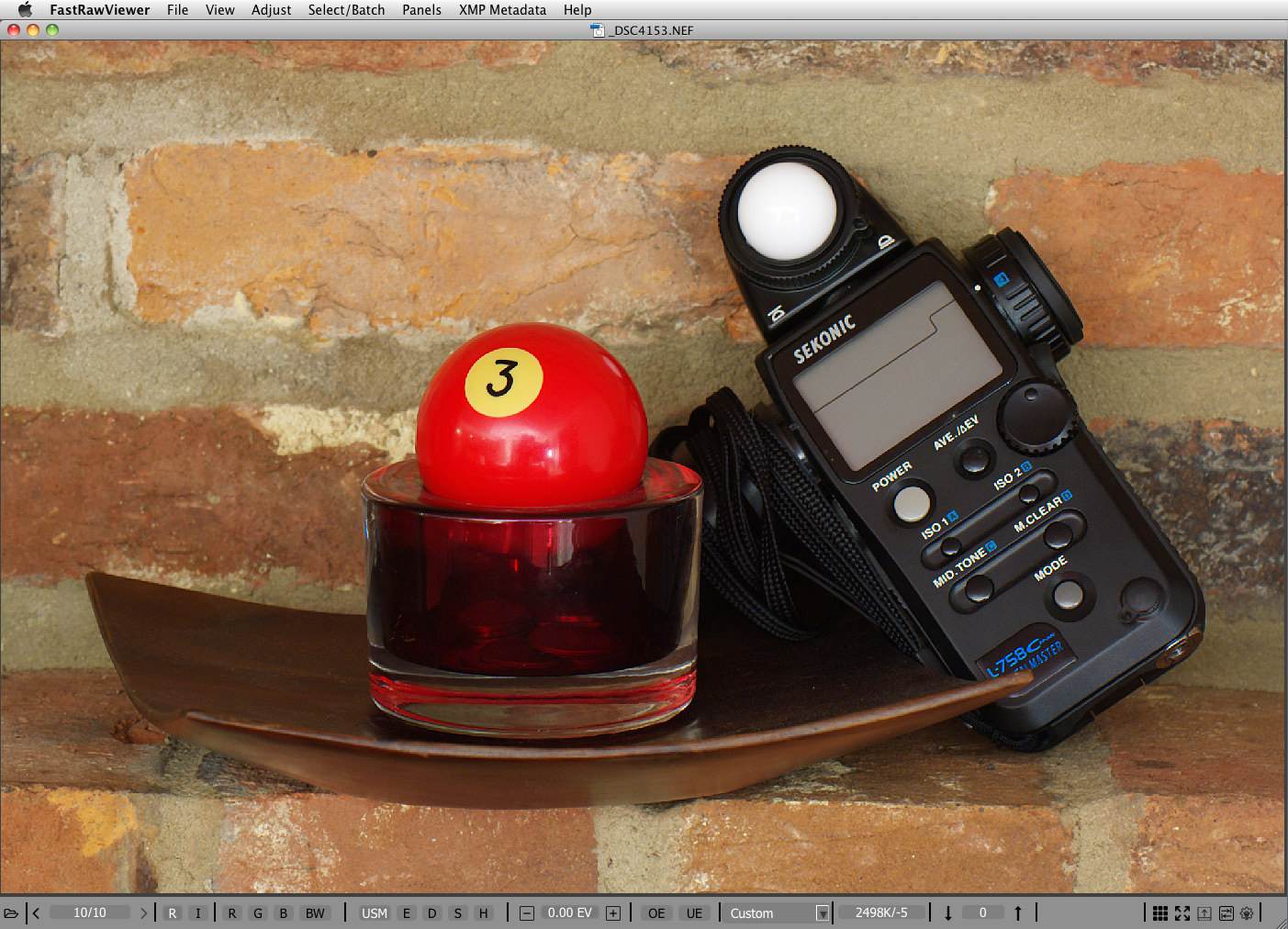
We made two shots of the same scene – one (#4152) was exposed according to the in-camera exposure meter set to matrix metering mode. The other shot (#4153, Figure 1.) was exposed 1 2/3 EV hotter (spot-metered from white dome, for the procedure to determine the amount of correction please read on, or you can simply bracket). Matrix metering seems to have gotten fooled by the specular highlights on that white dome, hence it underexposed a little more than usual.
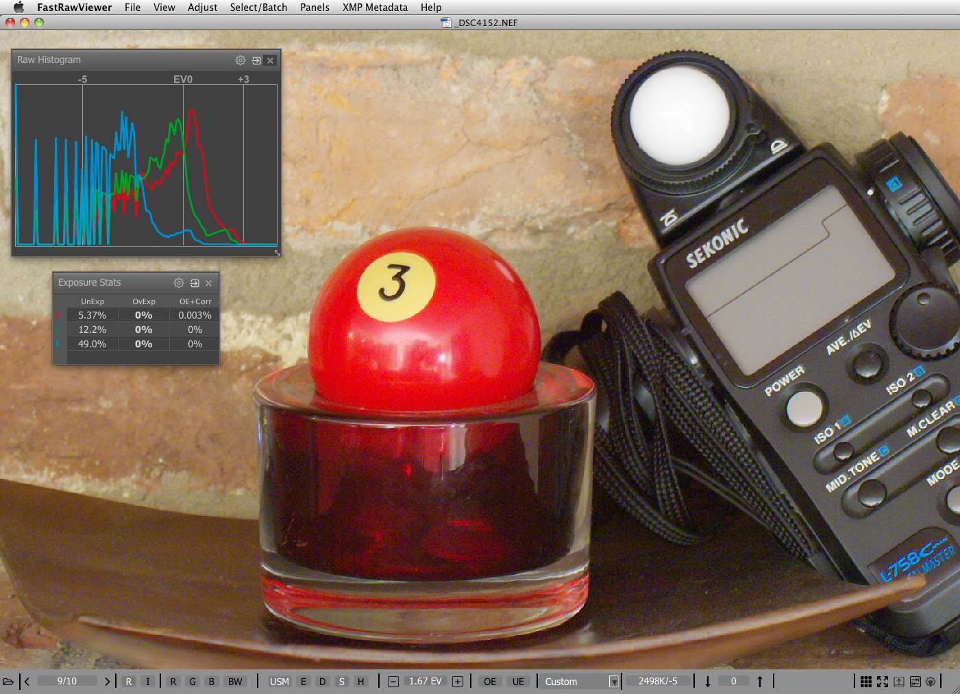
We opened them both in FastRawViewer, applied Shadow Boost to both of them to open the shadows, and applied +1.67 EV exposure correction to shot #4152 (the one that was exposed according to in-camera exposure meter recommendation, so that both of the shots had the same overall brightness).

As we can see on to the RAW histogram for shot #4153 (Figure 2) the capture definitely has more than 11 stops. Now we look at shot #4152.
As we can see, shot #4152 exhibits significant noise everywhere below midtone. The thing with a camera’s dynamic range is that those exciting numbers become valid only when the signal reaches the maximum; that is, the exposure is the hottest possible for the given camera at a given ISO. Imagine a bucket having a volume of 2 gallons. If you do not fill it up to the top, some volume is wasted. It’s the same with a camera. If your whitest white is not exposed to the maximum, the top portion of the dynamic range is not being used. This immediately means that in order to use the dynamic range of the camera to its fullest and simultaneously to have as little shadow noise as possible, the whitest whites where you want to keep some texture details need to be exposed so that they are just below clipping. In a sense, one can say that dynamic range characterizes the depth, and starts from the top, while the bottom is sort of fuzzy because of individual tolerance to noise, viewing conditions, size of the output, etc.
Back to our bucket analogy – if one tries to pour, say, 2.5 gallons in it, an overflow happens, and half a gallon will end up on the floor. In digital photography we know this as highlight clipping. That is, if we try to expose a pixel hotter than its capacity allows, everything that is above the capacity will pour out, causing blown-out highlights. By the way, if one tries to set exposure low to keep from clipping all the light sources and specular highlights, he is, most probably, also wasting a couple of stops of dynamic range.
Unfortunately the metering systems of our cameras are not designed to provide the proper placement of the highlights right out of the box (this is partially because to do so, the camera’s AI needs to make a guess as to what a photographer considers to be “important highlights”, and if it guesses wrongly, it may arrive at an unacceptable exposure). One can try different metering modes with the camera, with mixed results when it comes to optimal exposure for RAW. You can use RawDigger or FastRawViewer to see how close you are; be prepared for more misses than hits, in part because the complex metering modes are optimized for JPEGs rather than for RAW. Reliability and repeatability, however, come with manual metering in the spot meter mode. While placing important highlights at the top, let’s take advantage of one very well-known and stable feature of the camera: cameras are calibrated in such a way as to provide the exposure that will result in the rendering of whatever was under the spot meter as “middle grey”.
For a JPEG middle grey is defined as 118 RGB in sRGB color space, which corresponds to the proverbial 18% grey (and L* = 50 in Lab color model, too). For RAW, middle grey is not fixed by common standards, and camera makers have some freedom while placing it. Why is this so? Modern cameras have relatively low noise, and customers often complain that the highlights in their exposures are blown out. To provide extra room for the highlights, camera makers tend to calibrate the exposure so that it shifts middle grey down to 13% (instead of 18%), and often even lower than that. This is what often causes the rumors that camera makers cheat with ISO. In fact it is not cheating, because in most cases the ISO speed is defined for the processed output (JPEG) and not for RAW. Lets look at the shots of the scene we have already used in the article “Why Bother Shooting RAW if Culling JPEGs?”.
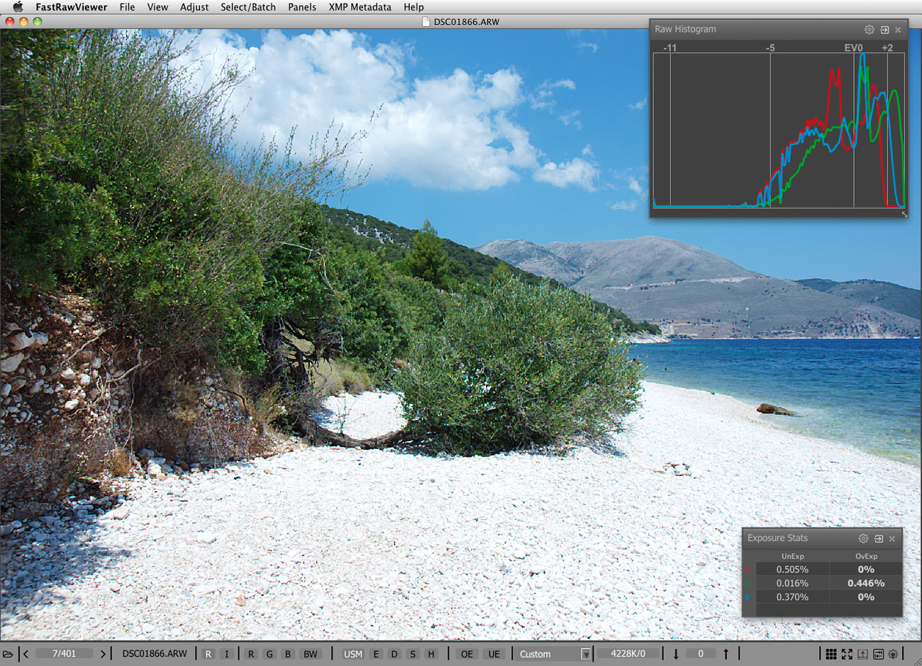
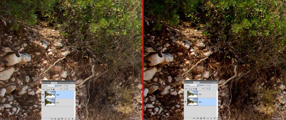
Shot #1861 was exposed according to the in-camera exposure meter and it has the hottest possible exposure for JPEG. Shot #1866 had exposure increased by 1 2/3 EV, and it has the optimal exposure for RAW (Exposing to the Right / ETTR). If we look at the shadows of those two shots after running them through ACR (shot #1866 was converted without any adjustments; while shot #1861 was converted with +1.67 exposure correction applied in ACR, to “match” the exposure difference between the shots), we see that there’s quite a difference in the shadows between these two shots. By the way, the smaller the sensor is, the more difference optimal exposure will make.
A tone curve applied when rendering a JPEG takes care of matching of whatever the middle grey is in RAW to the standard 18% grey in JPEG. But if we are shooting RAW and trying to exploit the dynamic range of our cameras to its full potential we need to set an exposure which is close to optimal, and place the highlights in the RAW where they belong – at the top of the dynamic range of your camera.
In other words, the top of the dynamic range of the scene (and by scene we mean everything you want to capture, and not the irrelevant / specular highlights) needs to be placed at the top of the dynamic range of the camera.
Back to the question of achieving this goal in a reliable and repeatable manner:
- First, we need to know the value for the middle grey in RAW numbers. This varies by camera model and sometimes by ISO setting.
- Next we need to know the maximum value that the RAW file may contain. This also varies by camera model and may depend on ISO setting; it may be the same as the maximum value for ADC (12 bits, 4095; 14 bits, 16383), or it may be less.
- Finally we need to calculate the result – the number of stops between the middle grey in RAW and the maximum in RAW for this specific camera and given ISO setting, to use this number as the exposure compensation when metering off the highlights that we want to keep.
Again, to use the result we need to meter from the whitest white in the scene where we want to preserve some texture and details, and apply exposure compensation in the camera that equals the number we have just determined. Consequently, the important whitest whites of the scene will receive the maximum allowed exposure, thus being placed at the top of the dynamic rage of the camera. This way you have achieved optimal exposure, also known as ETTR. The whole thing hinges on the theory that whatever is presented to an exposure meter will be recorded as middle grey as soon as the exposure meter recommendations are followed. Let’s check this theory.
We made six shots of the ColorChecker (Figure 1):
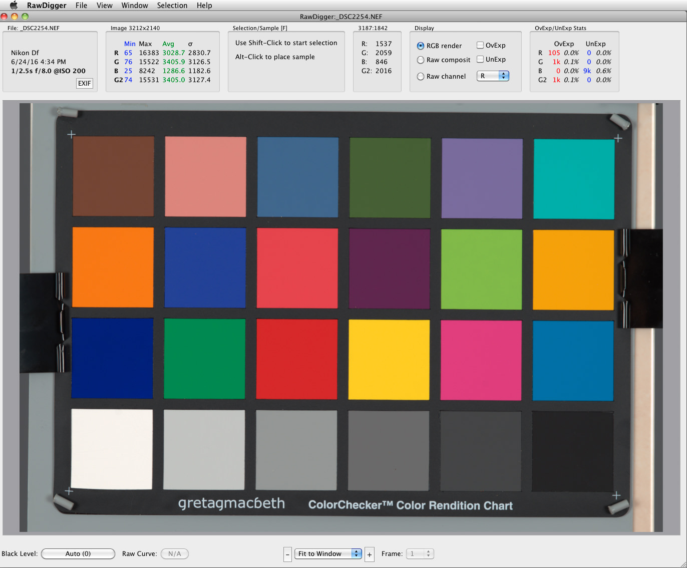
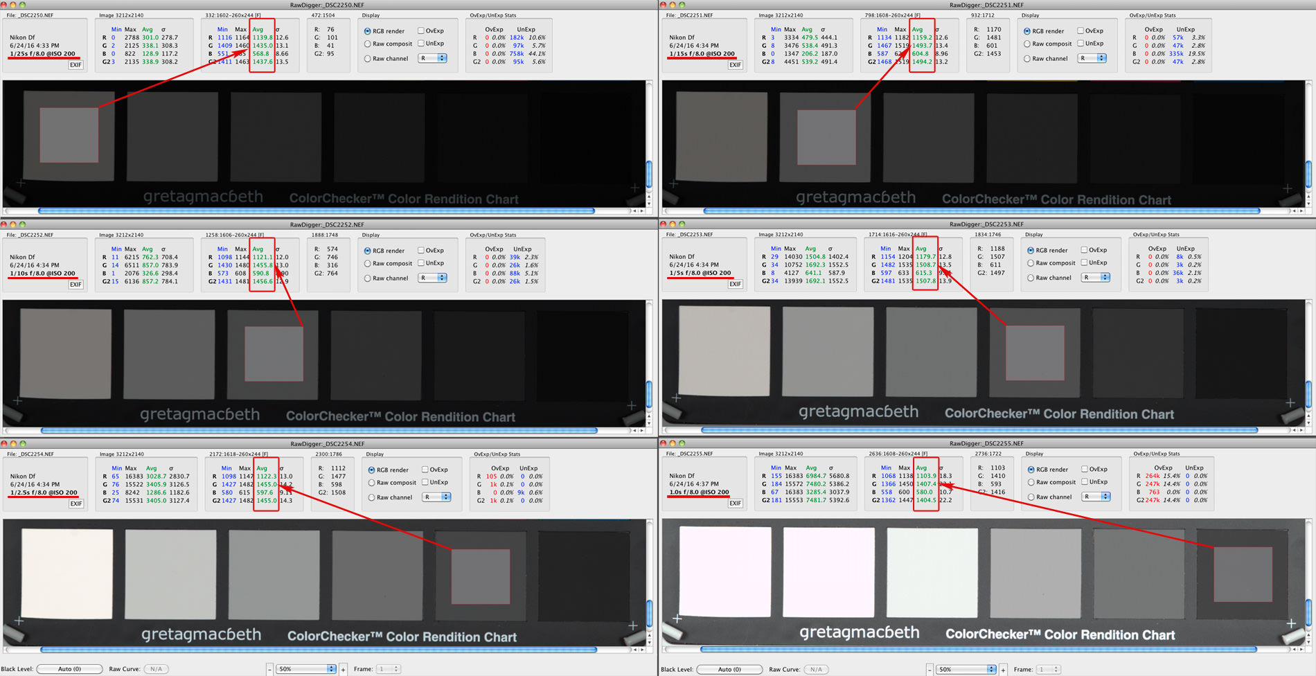
For each shot, we spot-metered one of those neutral grey patches at the bottom row, starting from the white patch, setting the exposure according to the recommendations of the spot meter. Next, we opened those shots one by one in RawDigger, sampled the patch we spot-metered, and checked the RAW values for this sample.
As you can see, the RAW values for the patch under the meter are very close to each other:
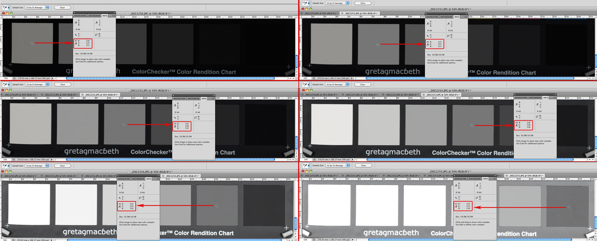
Because the camera was set to record both RAW and JPEG, we can check the RGB values in Photoshop too. As expected, they also turned to be very close to each other and to the target value for the mid-tone for JPEG, RGB=118.
Now that we are confident that the spot meter indeed guides the exposure in such a way that whatever shade of grey we put under the spot meter, the result will be the same number in RAW, with the number representing middle grey in terms of camera calibration for RAW. Because the theory proves to be true, you don’t need to meter and shoot all 6 patches: one is enough, or you can use a grey card.
- To get the most accurate reading for the middle grey in RAW, it is more practical to use a light grey patch / card (ColorChecker Passport has a separate grey page for white balance, it has L*=81, or, in other words, it is 60% grey, bright enough to use with confidence) or matte white. The reason for using lighter tones is to keep flare as low as possible for both metering and capture. The higher reflection values of the lighter samples are less prone to flare compared to lower reflection values for dark grey and black samples.
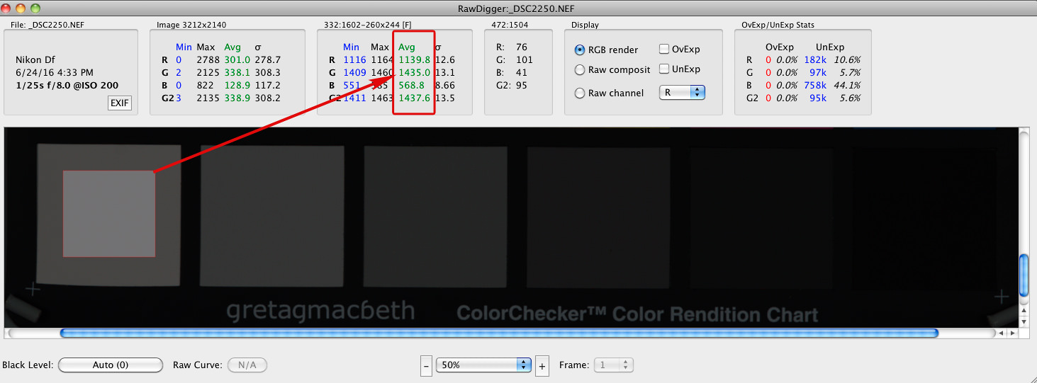
So to get GMiddleGrey, make a shot with exposure setting according to the spot meter recommendation for a white or a light grey patch, open the shot in RawDigger, place a sample on the patch from which you metered, and read average value for the Green channel, Avg G. In our case, GMiddleGrey = 1435.
- Now let’s determine the maximum value for the G channel that RAW can contain (maximum values may be different for different channels).
There are basically 2 ways to determine the maximum:- One way, which does not require additional shots, is to include from the beginning some source of relatively small specular highlights in the scene (a shiny metal ball, for example, is what is often used); however, this can create flare in the shot, and that flare will throw the metering off; maybe just a little, but sometimes significantly.
- The other way is to simply shoot with long exposure, ensuring that part of the shot reaches clipping.
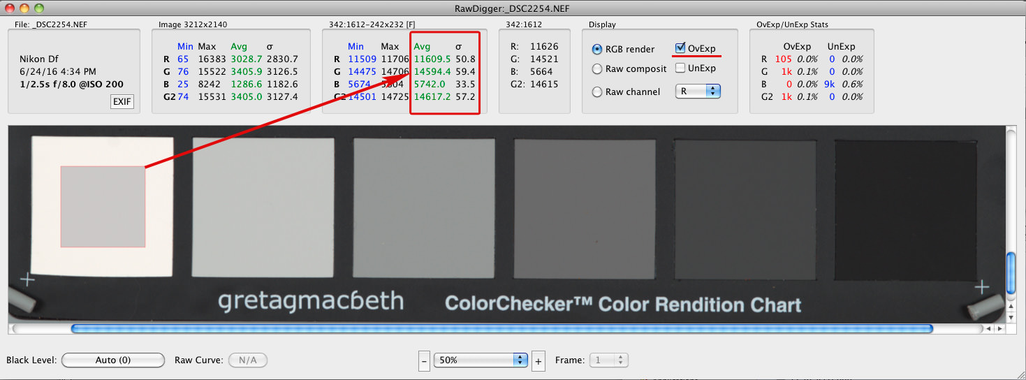
The truly clipped region will usually have a very small sigma (σ, standard deviation, Std.Dev.) value, in the order of single digits, in many cases very close to 0. The mean (average, Avg) value of the green channel for the clipped region is the maximum raw value we are after. On Figure 5, the average for green (Avg G) is 14,594.4; the standard deviation for green (σG) is 59.4. This means that there is no clipping.
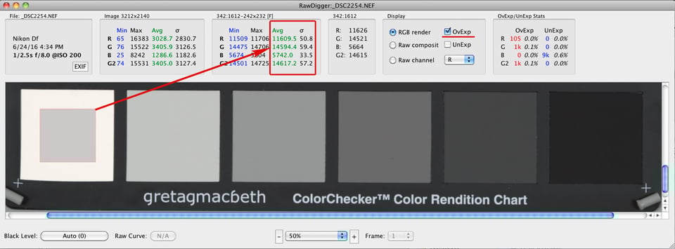
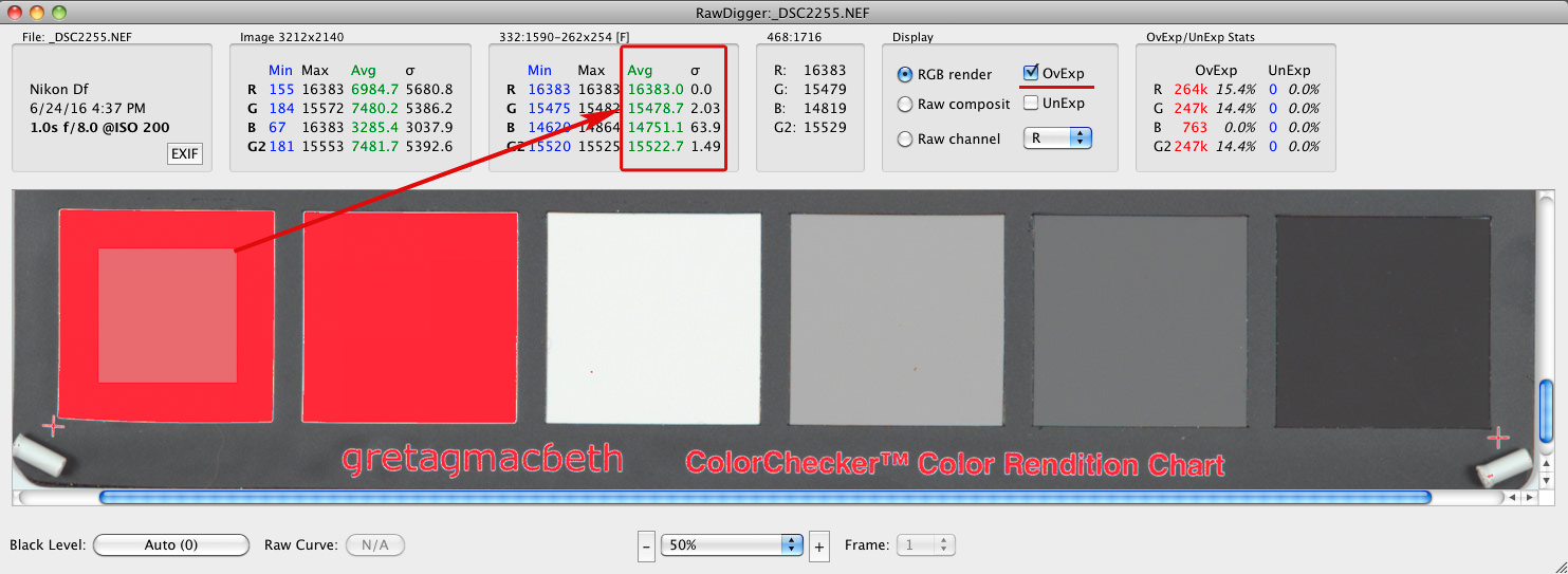
Figure 10 – RawDigger. Shot #2254. Large sigma (σ) values for all channels On Figure 6, the average for green (Avg G) is 15,478.7; the standard deviation for green (σG) is 2.03. That is the G channel clipping all right, and increasing exposure further will not help decrease σG in any significant manner – see the next Figure, #7.
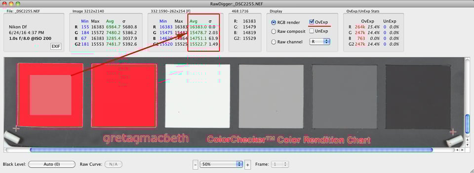
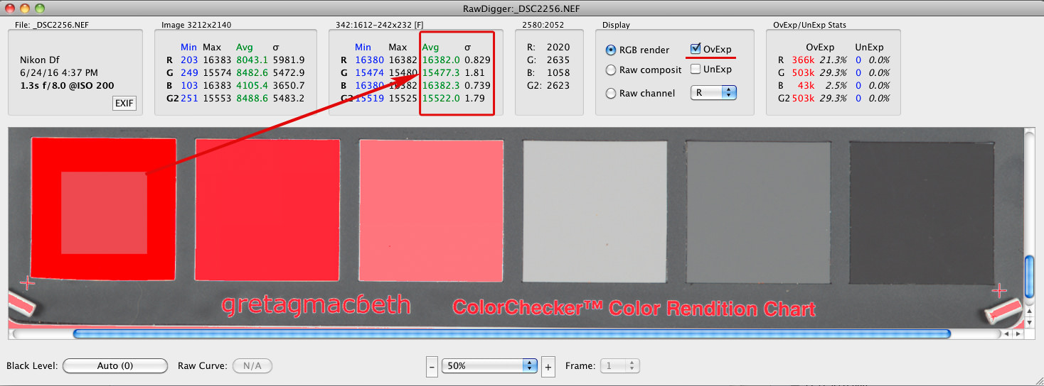
Figure 11 – RawDigger. Shot #2255. Small sigma (σ) value in Green (and Red) channels On Figure 7, the average for green (Avg G) is 15,477.3; the standard deviation for green (σG) is 1.81; that is, the green channel G is clipped, like it is on the previous one:
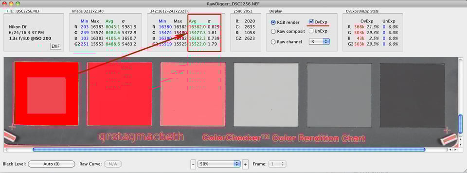
Figure 12 – RawDigger. Shot #2256. Small sigma (σ) values in all channels Nevertheless, the Avg G from the previous shot, #2255 (Figure 6) is a better choice: as you can see the Avg G is larger here, and this is because we triggered intense anti-blooming on shot #2256 (Figure 7), and it acts like solarisation, also known as a Sabattier effect. On film, increasing exposure results in decreased density of the negative; however, it is much milder on digital.
So, we will consider Avg G for a sample area from shot #2255 (Figure 6) as maximum raw value: Gmax = 15,478.7
- Finally, let’s calculate the value of exposure compensation (the number of stops, EV, between the middle grey in RAW and maximum / clipping point in RAW) for the given camera at a given ISO. We are going to use the formula:
EV = log2(GMax / GMiddleGrey) (1)
If you are interested in what the corresponding percent of grey is, you can calculate it as
percent = 100% * GMiddleGrey / GMax (2)
In our case GMiddleGrey = 1435 and Gmax = 15,478.7, so using the formula (1) we get:
log2(15,478.7 / 1435) ≈ 3 1/3 EV
That is this value of exposure compensation turns to be +3 1/3 EV (meaning the calibration for our camera puts the mid-tone in raw to 9.27%, nearly a stop lower than the “expected” 18%).
Let’s shoot with calculated exposure compensation and see… For the next shot #2257, we metered off the white patch, applying to the meter readings the exposure compensation we just determined, +3 1/3 EV. Now we open it in RawDigger and check raw values of the white patch:

As you can see, for a white patch average RAW value for Green channel (Gavg) is 14592.5. That is we are very close to the clipping point but still below it.
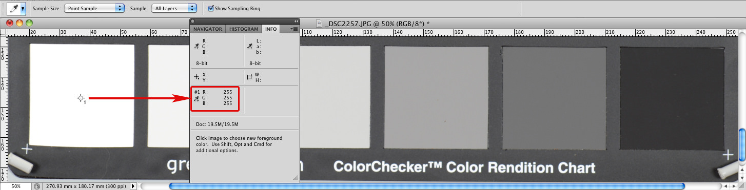
If we look at the JPEG of the shot #2257 (Figure 9) we will see that we “overexposed”: R=G=B=255. That is, of course, not so. OOC JPEGs do not use the full dynamic range available in RAW.
If you hate calculations, you can use a brute force approach. Shoot some neutral patch or grey card, setting the exposure as per your camera’s spot-meter recommendations and start adding exposure compensation, EC (you can set EC initially to +2 1/3 EV, which corresponds to calibration of the mid-tone in raw to 20% grey; we suggest this because calibration shouldn’t be higher than 20%) until the raw values for the patch or card comes close to clipping, within 1/3 EV from it.
Incidentally, you can often hear advice to meter off of the 18% grey card to set the correct exposure. This exposure is not likely to be optimal for raw, as in most cases it does not place the highlights high enough on the DR scale, but let’s check it.
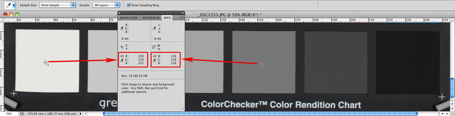
Shot #2253 was metered from the N5 patch of ColorChecker (which by design has L*=50, or, in other words, it is 18% grey) with zero exposure compensation. As you can see in RawDigger, the white patch is recorded 1 stop below clipping, and we have not achieved optimal exposure (Figure 10). Not even close.

If we check OOC JPEG for the same shot (Figure 11) we will see that while middle grey was correctly placed at 118 (sample 2), the RGB values for the white patch (sample 1) are (220, 220, 225), that is, seriously below maximum value.
Sekonic 758 in incident metering mode recommended 1/4s for shutter speed, matrix and center-weighted metering in the camera suggested 1/6s and 1/5s, respectively, while the shutter speed for ETTR, as we already know from shot #2257, is 1/2.5s. All out-of-the-box metering turned to be inefficient in terms of ETTR, but very consistent with the ≈1 EV difference we observed between calibration for raw for this camera (≈9%) and calibration for JPEG (≈18%).
We are very happy to hear that a new camera has ½ of a stop more DR than a previous model. We consider those ½ stop to be a huge improvement. However, if we are not using ETTR, we will be getting from this new camera the same or even lower image quality an ETTR practitioner is getting from the previous model.
Hi Iliah! This is a very illuminating article. Always knew about ETTR, but your method of computing the EV correction to be added over the spot metered value is a beautiful one that starts from first principles. What’s more, it is a one time thing to get the EV correction value
A question popped in my head that I could resolve after some thinking, but it might make sense to add that explanation above for completeness:
Why pick the 18% Grey’s Green channel value for your computation when the readings differs from the other channels so much (Red’s lower, Blue’s almost a 3rd)? Well I think that’s because the Green channel value is the highest among 18% Grey’s channel readings and your aim is to compute the lowest EV correction that does not blow the highlights for any of the channels
Also is there a way to figure out how many stops to lower in post processing other than to take and preserve another shot at realistic exposure? Given your site’s understandable distrust of camera tools (histograms, blinkies, etc. – they are tuned for JPEGs), I can’t think of a better one. Seems a bit wasteful in terms of memory to keep one raw image for every other just to match exposures
Hello.
After reading a lot about ETTR and UniWB, I decided to give it a try. At first I made a custom UniWB profile and a fitting picture-control setting for my D7200. Then I shot the same scene (under same conditions) with 3 different settings.
1) With Auto1 WB from camera, PC=FLAT, spot metering and +/- 0 EV.
2) With UniWB, custom PC, spot metering and +/- 0 EV.
3) With UniWB, custom PC, spot metering and + 2 EV (as ETTR “margin” by camera histogram)
After that, I analysed them with RawDigger and did some basic adjustments in Capture NX-D…
And, of course, the 3rd picture was (far way) the best! Not just in shadows, but also in highlights. RawDigger’s histogram indicated me that I used the sensors capacity as much as possible for this scene. When the other 2 shots were sunken in the dark on the left side. In direct comparison, after finished processing in CNX-D, they looked like from different worlds.
By chance I took a look at the file-sizes – 24MB (NEF 1 and 2) vs. 30MB (NEF 3) – which was another indicator to me that this method really works. 6MB more data captured by the sensor (without noticeable clipping in any direction) must be visible in the result – and it was!
On basis of this “eye-opening-experience” I continue to follow this way. Even with small greenish LCD-preview-pic beside the LRGB-histogram on my camera…
An excellent informative article and learnt more from comments section than from the main article , got cleared lot of misunderstandings of the concepts and doubts. The complete article including comments is great and informative including Betty’s clarifications on the subject except the unnecessary silly issues. Clearly Harvey did not know the difference between various metering modes and meter readings or might have misunderstood the subject, if that is the case ,there is noting wrong in accepting it , instead of diverting the to the discussion something else. Let me thank Iliah Borg, Nasim, Pete A and Betty for the most informative article and comments. Hope to see many more such articles.
KVS Setty: There is nothing wrong with my understanding of metering modes and meter readings. Don’t know why you need to poke your head into an old silly argument.
Peter, are you suggesting that I was having a conversation with myself?
I should add that my initial comment to Betty, which was about her condescending tone, was not a point of contention. The only debate that ensued from that was between Betty and Kevin regarding the identity of Betty’s gender. Further, the fact that Betty omitted Kevin’s name from the group of names she listed is evident that she was not referring to those comments.
Additionally, Pete, now that you are sticking your head into this, I don’t believe that initiated any conversation with you. I did not pick a fight with you.
“Peter, are you suggesting that I was having a conversation with myself?”
It does seem that way.
Much better for all concerned.
“I should add that my initial comment to Betty, which was about her condescending tone, was not a point of contention.’
It was to me.
I found it very hurtful…I had to take an extra Prozac to take the pain away…?
“Additionally, Pete, now that you are sticking your head into this…”
Pete has my permission to stick his head into this. His head is filled with wisdom.
On the other hand Harvey, your head is filled with brown stuff and it would be better if you stuck it back where it came from.
Hope the above is not too condescending…?
Pete, I said that Betty was the “one who first addressed me on the debate”. The operative words being “on the debate”. She stuck her head into my discussion between Iliah.
Harvey
PL is a global forum.
If you want to engage in private debate, stay off the internet.
Yes, I am aware that it is a public forum. Sadly, I allowed myself to get dragged into a childish debate in a public forum. That’s not something that Betty or I should be proud of. It does not look good on Photography Life either.
Harvey
“Yes, I am aware that it is a public forum.”
Good, then in future, you will, I hope, accept that comment from any quarter is OK.
The only childish part of this debate was not so much your being plain wrong on a scientific/photographic subject, or even your not taking the opportunity to learn, but that you instead chose to try to prove yourself right by picking a semantic fight with an acknowledged expert in his field of expertise! How silly is that.
– And of course your subsequent peevish whingeing, squirming and abusiveness to divert attention from the fact that you were in a hole.
“The only childish part…”. That is your opinion. An opinion which is blind to your narcisstic behaviour.
How do you know what I have, and have not, learned? Do you possess a special device that can read the knowledge base in my brain? But of course a narcissist does not need such a device.
I did not pick a fight with Iliah. We had a discussion, which he, smartly, long gave up.
Harvey
“The only childish part…”. That is your opinion”
Yes Harvey, it’s my opinion; that a half baked amateur trying to prove an expert wrong on his own subject is about as silly as it gets.
I don’t see what my narcissism has to do with it.
“How do you know what I have, and have not, learned?”
I don’t, but hope springs eternal and will perhaps this time triumph over reality.
Fingers crossed.
“Do you possess a special device that can read the knowledge base in my brain?”
No special device needed.
A plank is a plank – plain for all to see.
“I did not pick a fight with Iliah. We had a discussion, which he, smartly, long gave up.”
Call it what you will.
He told you, more than once, that you were flat wrong.
He smartly gave up because trying to educate a plank is futile.
I was not attempting to prove Iliah “wrong”. Rather, he was attempting to prove me wrong, based on a technicality that lacked context. The fact that our final contentious point was the definition of “semantics”, rather than my assertion that meter readings are dependent on the metering mode, is evidence to what I have said. Iliah never disputed the fact that meter readings are dependent on the metering mode.
“The first step toward change is awareness. The second step is acceptance”, Nathaniel Branden.
You have made the first steps in your recovery from narcissism. Good on you.
Harvey
Stop rewriting history.
Brush up your photography.
Don’t worry about me, I will be just fine.
“I was not attempting to prove Iliah “wrong”. Rather, he was attempting to prove me wrong, based on a technicality that lacked context.”
…..Iliah was attempting to prove you wrong….Yeah, right…….?
Iliah never disputed the fact that meter readings are dependent on the metering mode.
“The adjustments take place based on meter readings, not mode.”
You are living in a parallel universe, a sort of LaLa land where memory and reality merge into delusion.
Meter readings don’t take place in a vacuum, independent of other variables. For the sake of exactitude, there are a number of variables, in the process, which both Iliah and failed to mention. So, perhaps we were both “not correct”. At no point did Iliah explain the process from A to Z.
At this point, who, other than Betty, cares if one, or both of us, was not correct. After all, to err is human. I have been incorrect on numerous matters numerous times in my life and I will be incorrect numerous times in the future. It is part of being human. No shame in that.
Your quote of Iliah was his initial point of contention, not his response to my follow up point, which he failed to answer head on, presumably because doing so would have been an admission that he was nitpicking, which would have been okay if he had taken the time to educate by explaining the process from A to Z. Unfortunately, he appeared to be more motivated in proving me “not correct” on a technicality, rather than educating. This is why we had a problem.
So, no, I do not live in a parallel universe.
The subject of Iliah’s article is more than adequately conveyed in the title of his article: How to Use the Full Dynamic Range of Your Camera.
The detailed explanation of the subject is more than adequately conveyed in the article itself and in Iliah’s replies to the readers who wish to learn.
It is impossible to explain any advanced concept, from ‘A to Z’, to people who have not only failed to understand steps A, B, C, and D; they also delight in taunting those of us who do fully understand the advanced concept from first principles.
Taunt away to your heart’s content — we really don’t mind because *this* universe is never going to alter its laws of physics to comply with *your* wishful thinking :-)
Harvey
“Meter readings don’t take place in a vacuum, independent of other variables.”
Strictly speaking Harvey, yes they do.
The only variable, as far as the meter is concerned, is the light falling on it.
You are utterly confused about the ‘other variables’ because you don’t understand the differences between metering, metering modes, calibration, exposure, ISO, and Auto ISO, nor how they relate (or don’t relate) to each other. Until you do, there is little point in your trying to engage in a discussion on photography, still less insult an expert with your idiotic, semantic nitpicking.
With regard to your complaint that “At no point did Iliah explain the process from A to Z.”… Iliah said:
“Dear Sir:
I answered your comments several times, with explanations. But this site is hardly a place to quote camera manuals at length. By the way, “adjusts the ISO based on the metering mode set in-camera” is not correct. The adjustments take place based on meter readings, not mode.”
You are lucky he was that polite.
‘The whole process’ was not explained to you because the article assumes more than a rudimentary grasp of photographic principles. When it became clear that you do not understand even the most basic terms used, there was little point in him wasting his time further or quoting a camera manual at you. RTFM Harvey.
It’s not Iliah’s job to teach you elementary photography from first principles in the middle of a discourse on ‘How to Use the Full Dynamic Range of your Camera’. If you want the ‘whole process’ to be explained to you, go and do the PL Level 1 Course and tell them there about all the ‘variables’ involved in metering.
Be prepared for laughter.
I had hoped that at some point in this, a light might have come on for you, but no, the fuse box has evidently blown and you seem content to sit whistling the intellectual equivalent of Yankee Doodle in the dark.
I just watched the 15 minute trailer for PL Level 1. There was not a single thing mentioned that I have not already learned.
Harvey
Learning is one thing, understanding is quite another.
Understanding has to pass the test of peer review and reproducibility.
Expert peers with impeccable credentials have told you you are wrong.
Reproducing what you have learned (about metering, metering mode and auto ISO) leads to a self evident nonsense.
Draw your own conclusions.
With respect, you need more than a 15 minute trailer.
“I just watched the 15 minute trailer for PL Level 1. There was not a single thing mentioned that I have not already learned.”
That which can be asserted without evidence, can be dismissed without evidence:
en.wikipedia.org/wiki/…%27s_razor
Again with the condescending tone. Can’t I say anything without drawing a personal attack?
Harvey
“Again with the condescending tone. Can’t I say anything without drawing a personal attack?”
You take care of your tone and I’ll take care of mine.
No personal attacks from me, Harvey. Just so we are clear:
A personal or ad hominem attack is an attack on the person rather than on their argument; most commonly on their character or some personal attribute such as physical appearance, character, gender, race, family background etc, with the aim of undermining their case without actually having to engage with it.
This is not be confused with an attack, no matter how vitriolic, humorous or sarcastic, on another’s argument, statements, actions or beliefs. Barbed writing is a legitimate tool in written debate and the fact that the recipient may take it personally or is offended, does not make it ad hominem.
Ad hominems are used by immature or unintelligent people because they are unable to counter their opponent using logic and reason.
For instance, the comments, “Betty, is it physically possible for you not to be such a huge jerk?” or “You are one angry, bitter, negative, condescending narcissist.” are good examples of ad hominem attacks.
Pete, this is not a court of law. I simply made a genuine comment. If you don’t believe it, that is your prerogative. I honestly don’t care. I don’t have to prove anything to you or anyone here. It’s not like I am trying to sell you, or anyone here, something, for which my credentials and knowledge base may come into question. My personal knowledge base is completely irrelevant to this website. I am not a contributing author here. So, nobody here should really give a darn what I do and do not know. It is not relevant to this site. I am simply a reader of this (and many other) site(s).
Better, suggested a course to me. My genuine reply implied that the course appears to have little to no benefit to me, based on what I already know. I find it sad that a genuine comment, draws such cynicism and criticism.
“My personal knowledge base is completely irrelevant to this website.”
I’m very glad that — after posting 42 tiresome comments on Iliah’s article — you have finally been able to accept the truth.
Harvey
That’s just an evasive, circular, self serving, apologia.
If you had made a genuine comment, you would have accepted the genuine explanations that Iliah, Pete and I offered. I wrote at least three quite detailed comments for you.
Your response, (besides expending an inordinate amount of energy criticising my ‘tone’), was to dismiss what been offered in good faith as ‘nitpicking’, ‘semantics’ and ‘silly banter’ while at the same time referring to me as a troll, a jerk and a narcissist; all the while insisting that your misguided contentions were correct and that Iliah was ‘just trying to prove you wrong’.
So finally you are right – this is not a court of law, you don’t have to prove anything, your knowledge base is completely irrelevant and nobody here really gives a darn what you do or do not know.
I did not know anybody was keeping score of the number of posts.
Harvey
Now you do.
Pete A is the kind of guy who puts a high value on accuracy.
“I did not know anybody was keeping score of the number of posts.”
No person is “keeping score of the number of posts”: the website server computer is displaying most, but not all, of your posts; and it is extraordinarily easy to ask a web browser to count the number of posts written by you.
Betty, I did not read a word you just wrote. You know why? I don’t care. Life is good and too short to waste bickering over nothing.
Harvey
“Betty, I did not read a word you just wrote.”
You wrote a reply to something you did not read?
I honestly don’t understand all the confusing, or am I confused?
What I know is that you want to have the histogram to the right as much as possible without clipping to get the highest SNR.
Dear Pim,
There are 2 caveats to what you’ve said.
First, having JPEG histogram on the back of your camera to the right is not enough, as you can see from www.fastrawviewer.com/culli…w-vs-jpegs the raw may still be very significantly underexposed.
Second, promoting the histogram to the right using ISO control does not have desired effect past certain ISO value, and is never an adequate compensation for low exposure.
Thanks for your reply, great article by the way.
Sure you need to use the histogram of the raw file actually. As for your second point, I think I dont understand ISO exactly, you mentioned earlier that there are camera models that decrease noise with raising ISO. Do you by any chance know where the technical details are explained behind this?
I would say that with raising the ISO, you double the amount of light and noise, and thus an increase of sqrt{2} in SNR…
Dear Pim,
ISO is an internal setting applied after the actual exposure took place, and as such it does not affect the amount of light. In the camera only shutter speed and aperture (exposure-time factors) control the light to the sensor. In auto exposure modes (except for Manual + Auto ISO) doubling ISO cuts the light in half.
Some cameras, mostly those that are based on Sony sensors, have very low read noise numbers at low ISO settings, thus raising ISO has very little effect on noise in shadows (read noise). However even with these cameras one still needs to be careful with the idea of shooting without adjusting ISO at all, as raising ISO 2-3 stops up from base helps decrease banding artifacts and shadow tint (magenta, usually), which is the result of black level drift.
Other cameras, like Canon dSLRs and most of current Nikon 1-digit bodies (including Df, but excluding D3X), have relatively high read noise levels at base ISO, and read noise goes down significantly with ISO going up to a certain point which is sometimes called “point of invariance”. The graphs on www.photonstophotos.net/Chart…Shadow.htm go very flat starting from that point of invariance.
Iliah,
Thanks a lot for your excellent article. I have been waiting for it ever since February and even feared you would never publish it due to the rather weary response to your midtone articles.
I have a couple of questions, though. In the article above you indicate that the exposure compensation value to be determined using your method depends on the camera model and possibly on the ISO value. Are there any ranges of ISO values with similar, comparable exposure compensation values for a given camera model? If yes, is there any shortcut for determining these ISO ranges (not the compensation values) for a given camera model, e.g. by using the sensor data published by Bill Claff (or do you even know these ranges for some camera models and are willing to publish them;-) ? If yes, how? I am just thinking about how to reduce the work to be done as well as the compensation values to remember to a manageable amount.
In addition to the excellent articles on PL, even the comments sections contain very useful and helpful hints, so I always try to read them. Although your article is about exposure, there are a lot of hints w.r.t. ISO in the comments above. Unfortunately, though, I do not understand them completely. And even after reading Bill Claff’s Sensor Analysis Primer (thanks for the link) I am still confused, especially w.r.t. PDR Shadow Improvement, which you also explained above.
Is my following interpretation correct? In case the dynamic range (DR) of a scene fits into the DR of a D810 at ISO 200, it is wise to use ISO 200 instead of ISO 64 (although the D810 as a larger DR at ISO 64) because below ISO 200 the PDR Shadow Improvement is less and above the PDR Shadow Improvement does not increase significantly (provided you expose to the right, as explained above). If this is correct, then it would be wise to set ISO to 3200 on a D5 (provided the DR of the scene fits in to the DR of the D5 at ISO 3200), which if find really puzzling. (Please excuse my awkward formulations. This is because I do not know what PDR Shadow Improvement really is, nor how it is defined nor in what unit it is measured.)
Iliah, how about writing an article on PL about ISO? Given my lack of understanding as well as the questions and quarrels above, this might be a good idea! (And no, Bill Claff’s Primer doesn’t suffice, for it does not explain the different photographic scenarios to consider.)
Dear Carsten,
> Thanks a lot for your excellent article.
Thank you for your kind words.
> I have been waiting for it ever since February and even feared you would never publish it due to the rather weary response to your midtone articles.
Sorry for the wait. As to the responses, in my experience they are not an accurate indicator of interest or attitude; on top of that, some things need to sink in, and that can take time: months and years.
> In the article above you indicate that the exposure compensation value to be determined using your method depends on the camera model and possibly on the ISO value.
First, let me be clear, it is not _my_ method ;) Metering for highlights is actually one of the things spot-meters were designed for; with film, one can observe the result directly to calculate the exposure shift (similar to the brute force approach I mentioned in the article), or one can use a densitometer (that is what RawDigger is for digital).
> Are there any ranges of ISO values with similar, comparable exposure compensation values for a given camera model?
Normally, camera metering (midpoint) is calibrated the same way for all ISO settings, leading to the same compensation value. Exceptions are: “Lo” settings (those are below the base ISO setting and are usually implemented through the shift of midpoint; in practice there is very little reason to use those, be it for raw or JPEG); some higher ISO settings, for example on Fujifilm cameras, also implemented as midpoint shift, but in the opposite direction, towards less exposure (no point in using those if one shoots raw); intermediate ISO settings on some cameras may need additional checking, see, for example, our article www.rawdigger.com/howto…so-setting
> In case the dynamic range (DR) of a scene fits into the DR of a D810 at ISO 200, it is wise to use ISO 200 instead of ISO 64 (although the D810 as a larger DR at ISO 64)
The first choice is to raise the exposure. That is, decrease shutter speed and/or open aperture up (ISO setting is not a part of exposure). The more light you allow onto the sensor during exposure, the lower the noise.
If the exposure can’t be increased further (because of considerations like shake, the speed of the subject’s movement, depth of field, risk of AF misses) it makes sense to start increasing the ISO. There are very few exceptions to this rule, but they are hard to analyse in a reply, and they probably merit a separate article, probably one not interesting to most.
Why would one increase ISO setting at all on ISO-less (ISO-invariant) cameras, or beyond the point of invariance (no further shadow improvement with the raising of the ISO setting)? – because read noise (and shadow improvement calculated from the decrease of read noise, measured in photographic stops on Bill’s site) is not all that matters when one starts to lift shadows, even for the best ISO-less cameras that are currently available. When the levels in shadows are scarce on EV scale, the relative error is large, resulting in black point drift, colour skews, banding, loss of contrast. Those problems are often not visible until we start to bring the shadows out. My rule of thumb is that for low light scenes, given that I’m limited by shutter speed and aperture, I set ISO about 2-3 stops above the point of invariance to ensure that the shadows are editable. If I’m not planning on opening the shadows, that’s another matter.
> it would be wise to set ISO to 3200 on a D5
D5 is not even close to ISO-less below the ISO setting of 2500. The colour in the shadows improves up to 2x of that, ISO 5000.
> how about writing an article on PL about ISO?
I have it in mind, but “The Arithmetic of White Balance and Why Should I Care” comes first ;)
> Normally, camera metering (midpoint) is calibrated the same way for all ISO settings, leading to the same compensation value.
Just one compensation value to determine and to remember – perfect.
> The first choice is to raise the exposure.
This is clear, for this is what your article above is all about. But was it? Apparently not, because for some reason I thought I could expose to the right at base ISO and then increase ISO to the point of invariance (i.e. ISO 200 for a D810, if I read the PDR Shadow Improvement data correctly) in order to improve the shadows. This would cause the highlights to clip, though. So, my interpretation explained above is just nonsense. Thanks for sorting this out.
> Why would one increase ISO setting at all on ISO-less (ISO-invariant) cameras, or beyond the point of invariance (no further shadow improvement with the raising of the ISO setting)? – because read noise […] is not all that matters when one starts to lift shadows.
Ok, since there are other contributing factors not reflected in the PDR Shadow Improvement data and since I do not know of any additional data showing them (and wouldn’t be able to interpret them correctly anyway), I am back to my previous mode of operation: having and using the ISO dial on my D810 makes sense – if I cannot further improve exposure, I will raise ISO in order get a properly “exposed” image and can then do whatever I want in post processing. See my last reply below, though. :-)
> D5 is not even close to ISO-less below the ISO setting of 2500. The colour in the shadows improves up to 2x of that, ISO 5000.
I just took a second look at the PDR Shadow Improvement data, and yes, the point of invariance seems to be at ISO 5000 with an improvement of almost 3 1/3 stops. Nevertheless, my original interpretation is nonsense.
> > how about writing an article on PL about ISO?
> I have it in mind, but “The Arithmetic of White Balance and Why Should I Care” comes first ;)
Deal – I will wait for both of them now.
> First, let me be clear, it is not _my_ method ;)
Sure, but you are the one who clearly describes this method and provides the tools needed ;)
Thank you mr. Borg for a very thorough, and insightful article.
Reading this thread this morning, it struck me, that being right often differs vastly from being polite or even just nice. It also is a great example of how to shut down debate. The article discusses (as far as I can see) how to best to utilize the dynamic range in a sensor. The condescending tone in various replies obscures this, and just leaves you sad.
Below is my sensored version of my deleted response.
Oxforddictionaries.com: “semantics: 1.1 The meaning of a word, phrase, or text: such quibbling over semantics may seem petty stuff”.
Merriam-Webster.com: “SEMANTICS: the meanings of words and phrases in a particular context”.
When debates lack “context” they can become “petty”.
Hopefully, this sensored version does not get deleted.
whinge [verb]: complain persistently and in a peevish or irritating way.
Pete, I just learned a new word. Thanks.
Next time a police officer pulls me over for speeding, perhaps I ought to borrow a page from Iliah’s book of logic and argue that the speed of the car was not dependent on me because the engine was blind to me and my foot. The trouble with such an argument is that I will get laughed out of court.
Harvey
A car, like a camera, requires intelligent input.
Without that, all bets are off.
When I first learned how to drive, I did go online to find out how the engine, clutch etc roughly work…
Why was my response deleted?